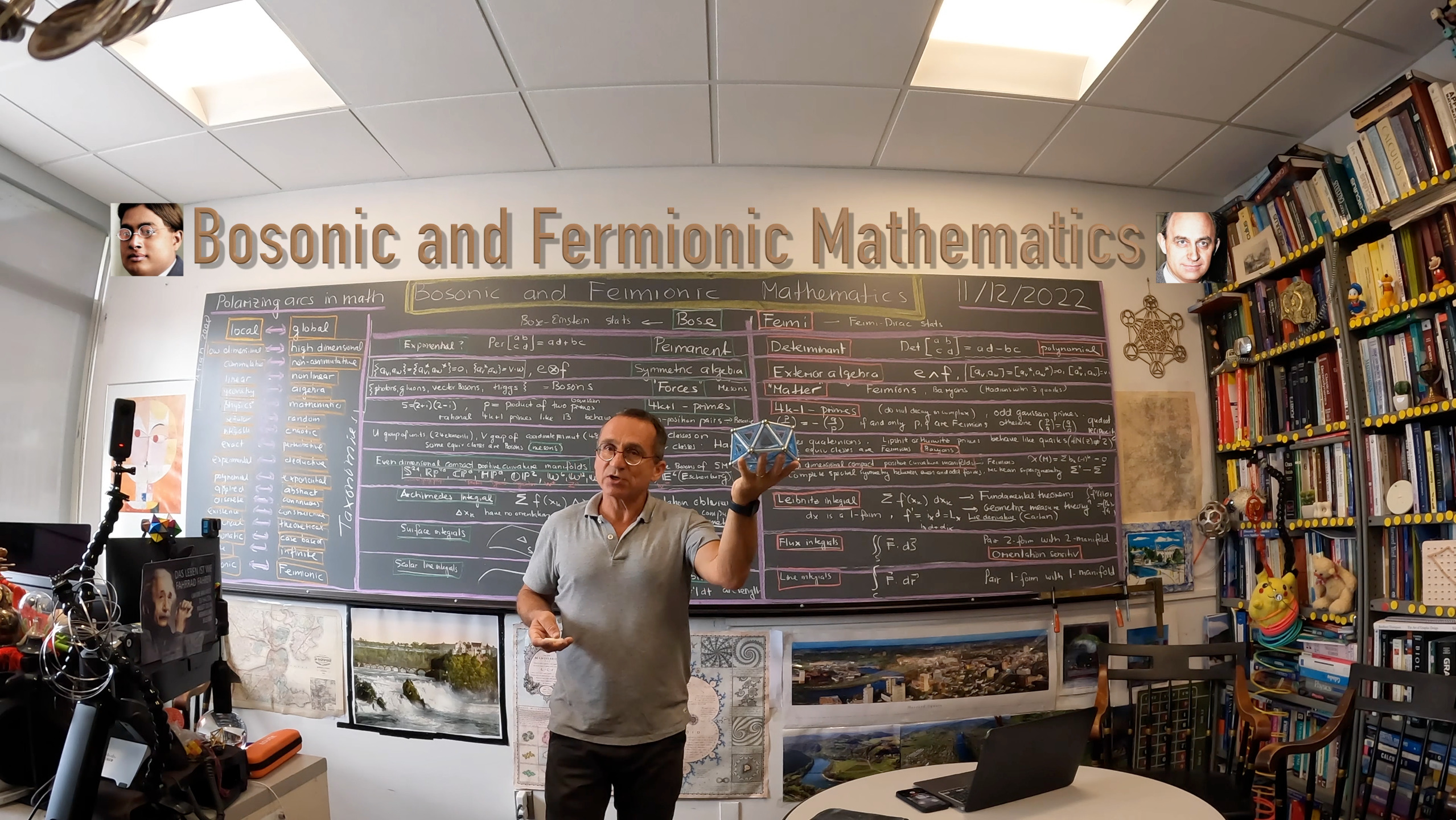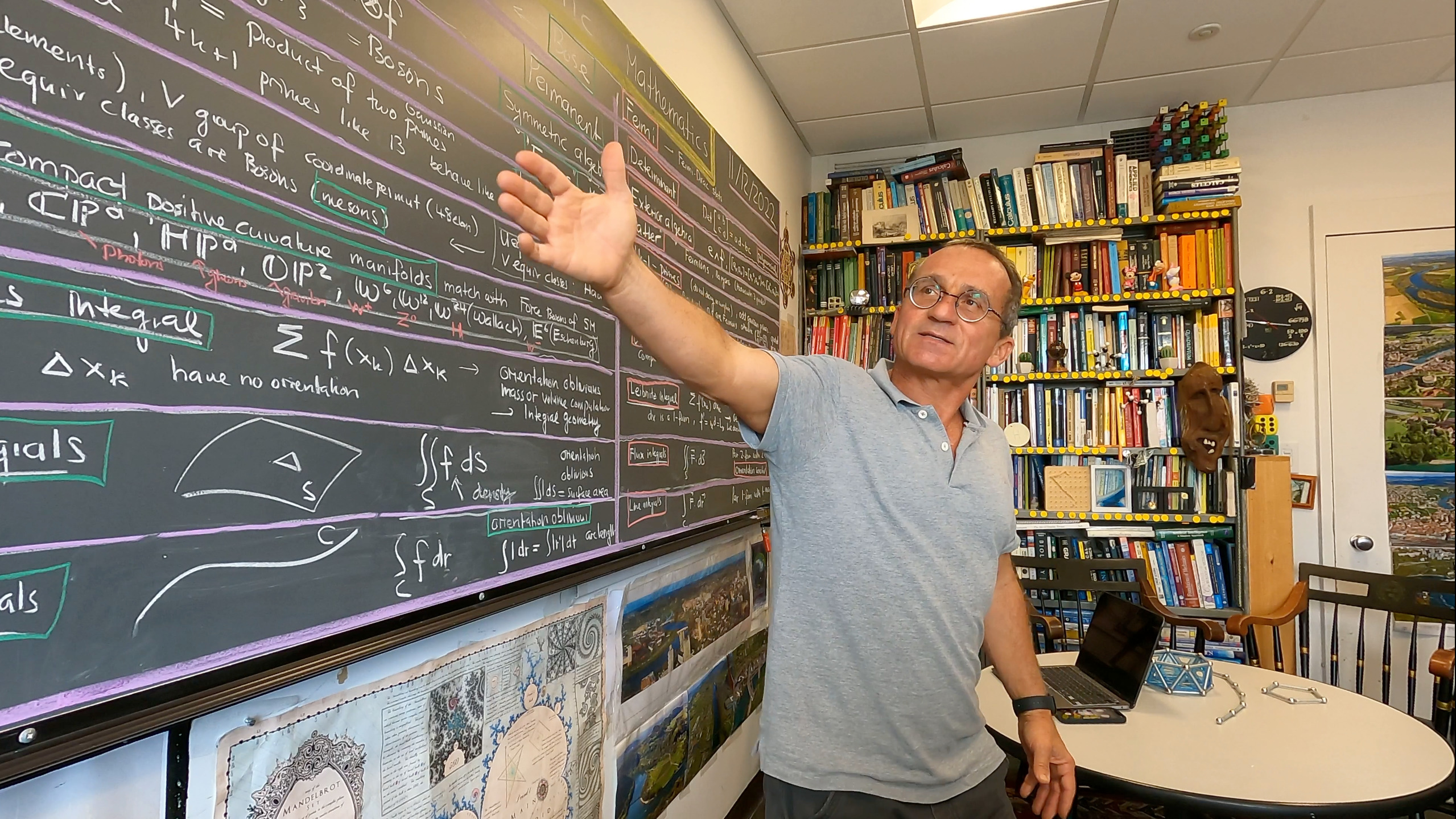
Bosonic and Fermionic Features in Mathematics

Even or odd, symmetric or anti-symmetric, integer or half integer, measures or de Rham currents, densities or differential forms, undirected or directed, orientation oblivious, or orientation sensitive, primes of the form 4k+1 or primes of the form 4k-1, permanents or determinants: there are many notions of mathematics which can be labeled either “Bosonic” or “Fermionic”. By the unreasonable of effectiveness of mathematics (a phrase of Eugene Wigner which echos sentiments from antiquity like the Pythagoreans or early modern scientists like Kepler and the mathematical universe hypothesis it would be natural to assume that Bosonic and Fermionic features also appear in nature. It is the other way round: we observe structure like Bosons or Fermions in nature, make mathematical models, extend the theorem is and then project them back (*). I think it is helpful to be aware about the Boson-Fermion taxonomy, especially in calculus. There are different integrals and derivatives appear in calculus. Calculus is mostly a Fermionic topic if the fundamental theorem of calculus is considered. Other parts are more Bosonic especially if integrating densities is a big deal. In multivariable calculus, especially when dealing with objects in space where the orientation is not obvious, we deal with both. When looking at surface integrals (these are integrals generalizing surface area) or scalar line integrals (integrals generalizing arc length) or volumes or mass computations, we do not care about orientation. when looking at line integrals or flux integrals, we do care about orientation. In other parts of mathematics like complex analysis or differential geometry this comes up more transparently. There are different approaches to the difficulty. One can chose not to include scalar line integrals and scalar surface integrals (which are Bosonic notions close to arc length and surface area) and focus on line integrals and flux integrals which both lead to the fundamental theorem of calculus. In single variable calculus, one silently gets from the 1-form f’dx to the 0-form f’ and morphs the exterior derivative d to a Lie derivative $L_X = i_X d$ which is in one dimensions equivalent to $L_X = (i_X + d)^2$ . The Lie derivative is an operation which can be defined for any differential form. It maps a k-form to a k-form similarly as the Laplacian does. This expression is due to Ellie Cartan. One can see this as a way to morph a Fermionic notion (exterior derivative) to something Bosonic (Lie derivative).

In an introduction course like multi-variable calculus one has to hide it under the rug, ignores the issue. One can also try to link the two things together in a more pedagogical way. One can for example write the line integral $\int_a^b F(r(t)) . r'(t) dt$ as $\int_a^b f(r(t)) |r'(t)| dt$ , where $f(r(t)) = F(r(t)) . r'(t)/|r'(t)|$ is a scalar function treated like a density. Cartan would have seen this as $f = i_X F$ , where X is the inner derivative mapping the 1-form F to a 0-form f. When integrating a scalar function like f over an interval, we are in an Archimedian setting and do not care about the orientation of the curve. The orientation of the curve has morphed via the interior derivative into the scalar function. For surfaces, the same is done for pedagogical reasons like in Stewart’s popular books. Because most teachers have learned calculus from Stewart, it remains a popular way to soften the flux integral issue. Mathematically, the mess is huge because one has to replace the 2-form $F dx dy$ with a scalar function but it is not possible to transcend from 2 forms to 0-forms. What textbook writers do is to upgrade the 2-form to a 3-form by taking an exterior derivative with a 1-form associated to the normal bundle then identify the 3-form with a 0-form. The hack goes like this: instead of computing $\iint_R F(r(u,v)) . r_u \times r_v du dv$ which is coordinate independent and can be pulled back along the parameterization to two dimensions, one introduces the scalar function $f(r(u,v)) = F(r(u,v)) . r_u \times r_v/|r_u \times r_v|$ , then can see the surface integral for $f$ as a flux integral: $\int_S F \cdot dS = \iint_R f(r(u,v)) |r_u \times r_v| dudv = \iint_S f dS$ . What happened is that that Fermionic orientation-sensitive flux integralhas become a Bosonic orientation oblivious scalar surface integral. The orientation has, similarly as before in the scalar line integral case been incorporated into the function f. The two-dimensional pedagogy hack makes use of that a surface can be embedded in three dimensional space. In reality, the flux integral does not depend on that and works verbatim also if the surface would have been embedded into a higher dimensional space. But one can adapt the choice of problems to this situation and produce situations where the hacked function f is simple so that you can compute flux integrals by knowing surface area.

Maybe I just repeat something here which I have pointed out a couple of times both in my work on graph theory as well as in courses like Math 22: if space is a graph G, we can integrate by counting things like counting the number of vertices, counting the number of edges or triangles etc. These are Bosonic counts, discrete Bosonic integrals. In order to make use of Fermionic notions and computations, one needs to orient the simplices. It is irrelevant how this is done. It is like putting a coordinate system in space. On a graph, we can even change the coordinate system when going from one simplex to an other. We do not need to have compatibility for neighboring simplices. If we have a discrete surface however, we usually like to orient the triangles in such a way that the orientations in the interior cancel out. This is the Fermi trick. In the interior, the Pauli principle annihilates space and only the boundary survives. Green’s or Stokes or the divergence theorem are now immediate. Why are they so hard in the continuum. One reason is that we can not access atomic higher dimensional parts of space easily without introducing sheaf theoretical notions.

Links: Mathematical Roots (notes 2010-2022) (PDF) , Bosonic and Fermonic calculus (blog 2016) (on this blog) , Positive curvature and Bosons (2020) (ArXiv), Some experiments in number theory (2016) ArXiv). For teaching here is my standard lecture on Stokes theorem, or the general Stokes theorem in arbitrary dimensions. For how calculus will be taught in 50 years (my standard quip in that matter), see this lecture on discrete calculus and something about discrete calculus in physics.