Gauss-Bonnet for Delta Sets

Finite geometric categories: graphs – simplicial complexes -simplicial sets – delta sets

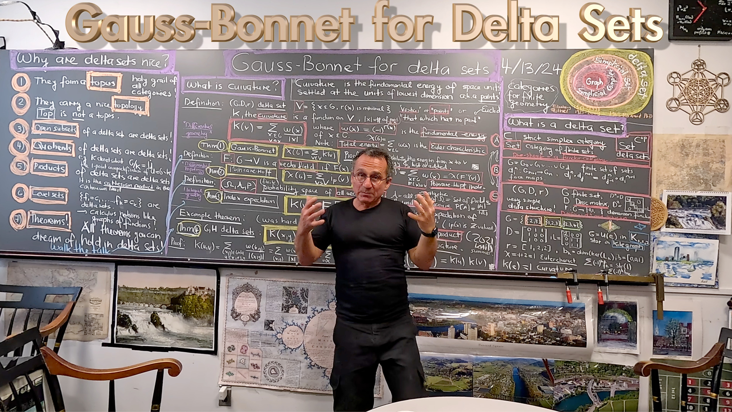
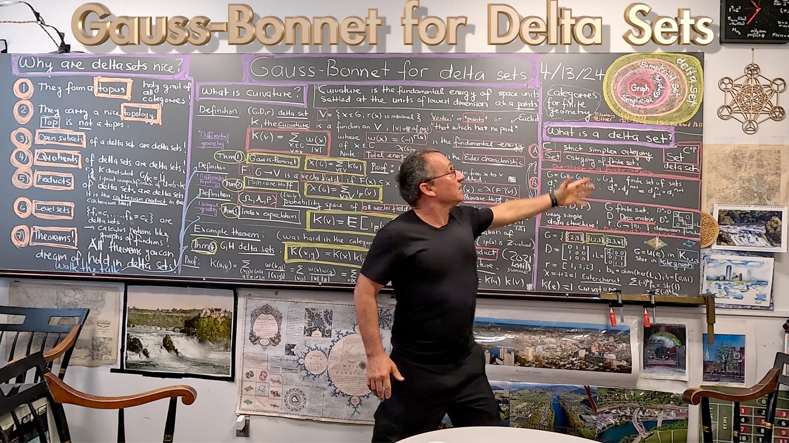
Delta sets were originally called semi-simplicial sets by Samuel Eilenberg and Joseph Zilber in 1950. Similarly than semi-rings are more general than rings or semi-groups are more general than groups, also delta sets are more general than simplicial sets. I myself tried for years to get an intuitive grip on simplicial sets only to realize that the more general structure of delta sets is easier to understand and more intuitive. There is literature claiming that simplicial sets are more general than delta sets but that is a misconception. You can find an argument about this here. These days, delta sets are introduced as the presheaf which is a functor category and a reasonable reason to scratch heads. While this serves a bit as a justification why the object is natural, I myself find it better to think about a delta set as a triple (G,D,r) where G is a set of n points, is a symmetric matrix with the property that is block diagonal compatible with the dimension function : the dimension function needs to be constant on each block of L. If G is a simplicial complex, a finite set of non-empty sets closed under the operation of taking finite non-empty subsets, then D and r can be derived from G. The dimension function in that particular case is just r(x)=|x|-1, where |x| is the number of points in x. In a simplicial complex, “points” are zero dimensional. In a delta set, the “points” (=”that which has no parts”) can have higher dimension. The smallest delta set is the initial object , where $[]$ is the matrix and r is the empty function; it is also called the void. Note that the empty set does not violate the assumption that every of its element is non-empty. it is custom to attach to the void the maximal dimension -1. One of the simplest delta sets is the set containing a single facet in a simplicial complex G of maximal dimension d. This is an open set as it is the star U(x) of the facet . If we define , then is the Euler characteristic of G. The k-th Betti number of a delta set G is the nullity of the k’th block of , meaning that the elements in that block have dimension . In the case of a single facet of dimension d only the block is non-empty, the other blocks are all empty. You see from this example already that we can not ditch the information in the dimension function . It was possible to do so for simplicial complexes, where every dimension below the maximal dimension is populated with simplices (by definition). The Betti vector of the facet is now $\latex (0,0,0,\dots, 1)$. The f-vector (counting how many elements there are of each dimension) of that delta set is also . Already interesting is the one-point compactification of the facet, which is the d-dimensional sphere. It can be described as the delta set with Betti vector $b=latex (1,0,\dots,0,1)$. It had always been a selling point for delta sets that we need much less cells. Here,l a d-sphere can be describe with 2 cells. When using simplicial complexes, we need cells as this is given as the boundary skeleton complex of a d+1 dimensional simplex. When using graphs (of course meaning simplicial complexes coming from graphs), we need already a complex with vertices and much more cells. Maybe the following table can serve as an advertisement, when we look at the smallest possible way to realize a 2-dimensional sphere in each category: . While the number of elements needed to describe a d-sphere grows exponentially in d both for simplicial complexes and graphs, the number of elements to describe a d-sphere within delta sets remains 2. Of course, the delta set representing the 2-sphere does not contain much structure, but it contains curvature. All the curvature is located on the zero dimensional part. For odd dimensional spheres, the curvature is constant 0 (this by the way is also true for simplicial complex or graph representations of all odd dimensional manifolds). For even dimensional spheres, the curvature is 2 and located on the zero dimensional point of the delta set. In the presentation from yesterday, I show how simple Gauss-Bonnet, Poincare-Hopf and Index expectation results are. This is one of my first attempts to popularize this point of view (january 2012). For index expectation, see February 2012. I tried myself to push this a bit into the continuum (like here in january 2020). At that time, I had reviewed a bit the Hopf conjectures and tried to get an experimental grip on them. The conjecture is that every even dimensional compact Riemannian manifold of positive curvature has positive Euler characteristic. An other conjecture is that there is no Riemannian metric on of positive curvature. Also this is an interesting theme for experimental math. One issue here is to define sectional curvature and so what “positive curvature” means for networks. We have no natural exponential maps in discrete manifolds. One reason to explore the Sard theme (which I wrote about in the last couple of months) was to make sense of what a 2-dimensional flat level surface through a point should be because then we have a notion of sectional curvature which is a realistic analog to the continuum notion. I once used the notion that every embedded wheel graph in the complex has positive curvature but this is very restrictive. This “sphere theorem” is very easy in that case. I call it a Mickey-Mouse Sphere theorem. Every sphere of positive curvature with that notion is a sphere. There are no projective spaces for example if the manifold should be implemented as the simplicial complex of a graph. In two dimensions, there are exactly 6 spheres. I wrote about this in my “parameters for teaching” paper which appeared in the book “A conversation on Professional Norms in Mathematics” from a workshop in 2019.

The port of the Gauss-Bonnet theorem or Poincare-Hopf theorem or Index expectation theorem (first probably explored by Thomas Banchoff in the continuum) from Graphs to Simplicial complexes and from Simplicial complexes to Delta sets is quite obvious: think about as the energy of an element . it should be obvious that most can be done also if this energy function is generalized to an arbitrary ring-valued function (energized complexes) but the case when even dimensional objects have energy 1 and odd-dimensional objects have energy -1 is the most common frame work. The Euler characteristic of G is then the total energy. An other important notion is the notion of a point in a delta set. Motivated by Euclid and pointless topology, we call a point an element in G “which has no part”. A point does not need to have zero dimension. It can be quite arbitrary. For stars U(x), (which are delta sets per se) there is only one point, the point x. Curvature is what happens if all the energy of space sinks in a diffusive way to the points. If |x| is the number of points in x, then w(x)/|x| is what each point in x “gets” when diffusing the energy to the points. Of course this diffusion process does not change the energy as nothing gets lost nor generated. Gauss-Bonnet is just a “conservation law”. Now, how can this ridiculously simple result imply the deep Gauss-Bonnet-Chern result for even dimensional compact Riemannian manifolds? That theorem is hardly taught even in advanced differential geometry courses as it is “too hard”. I myself learned it from the book of Cycon-Froese-Kirsch and Simon because there had been plans for a pro-seminar on Patodi’s proof of the Gauss-Bonnet-Chern result. (I read the proof during a vacation in the Swiss alps. (Here is some footage from 2022 recorded in this beautiful place)) but the seminar did not take place as the topic is rather tough. The link between the discrete and the continuum is index expectation. While Gauss-Bonnet diffuses curvature equally to the points in each cell, we can use a “vector field” do target the energy to a specific point F(x) in x. In the case of gradient fields, the point F(x) is the minimum of f(v) for v in x. For every probability measure on vector fields, we have a curvature. This also works in the continuum: for every probability measure on the set of Morse functions (a good class because they have nice indices and no degeneracy). Now, any compact Riemannian manifold M can be isometrically embedded in an ambient Euclidean space E. This produces now a natural probability space of Morse functions as almost any linear function on E produces a Morse function on M. Taking the index expectation curvature is of course a curvature which satisfiies Gauss-Bonnet, as the expectation of functions adding up to Euler characteristic also produces a function producing Euler characteristic. The index expectation formula curvature has the property that it is invariant under rotations of the tangent space. Now, curvature is a local property and we can near a point x pretend that we have an embedded graph in an Euclidean space. The index expectation curvature K(x) is invariant under rotations in the tangent space . There is only one curvature which satisfies this property.

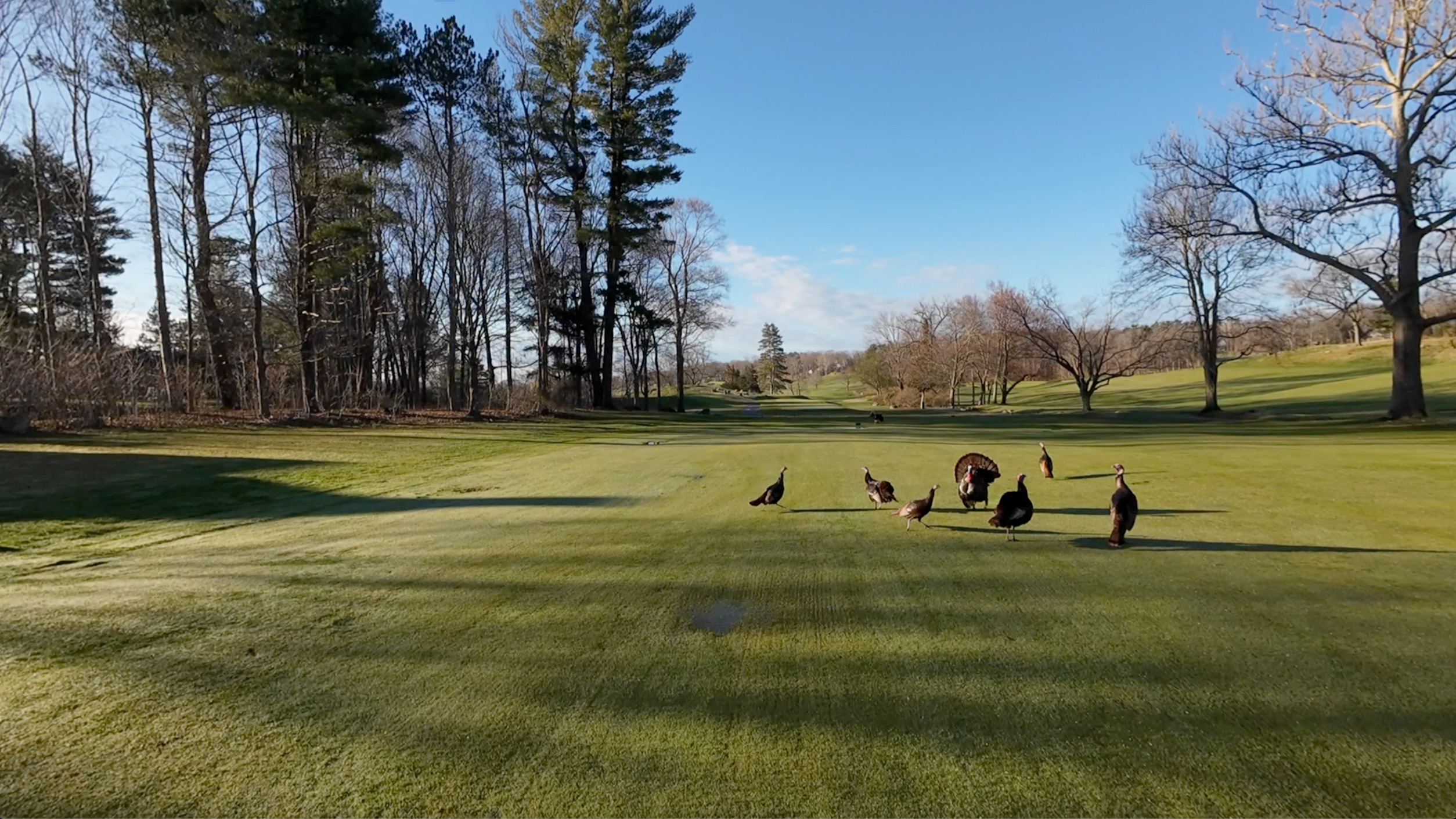
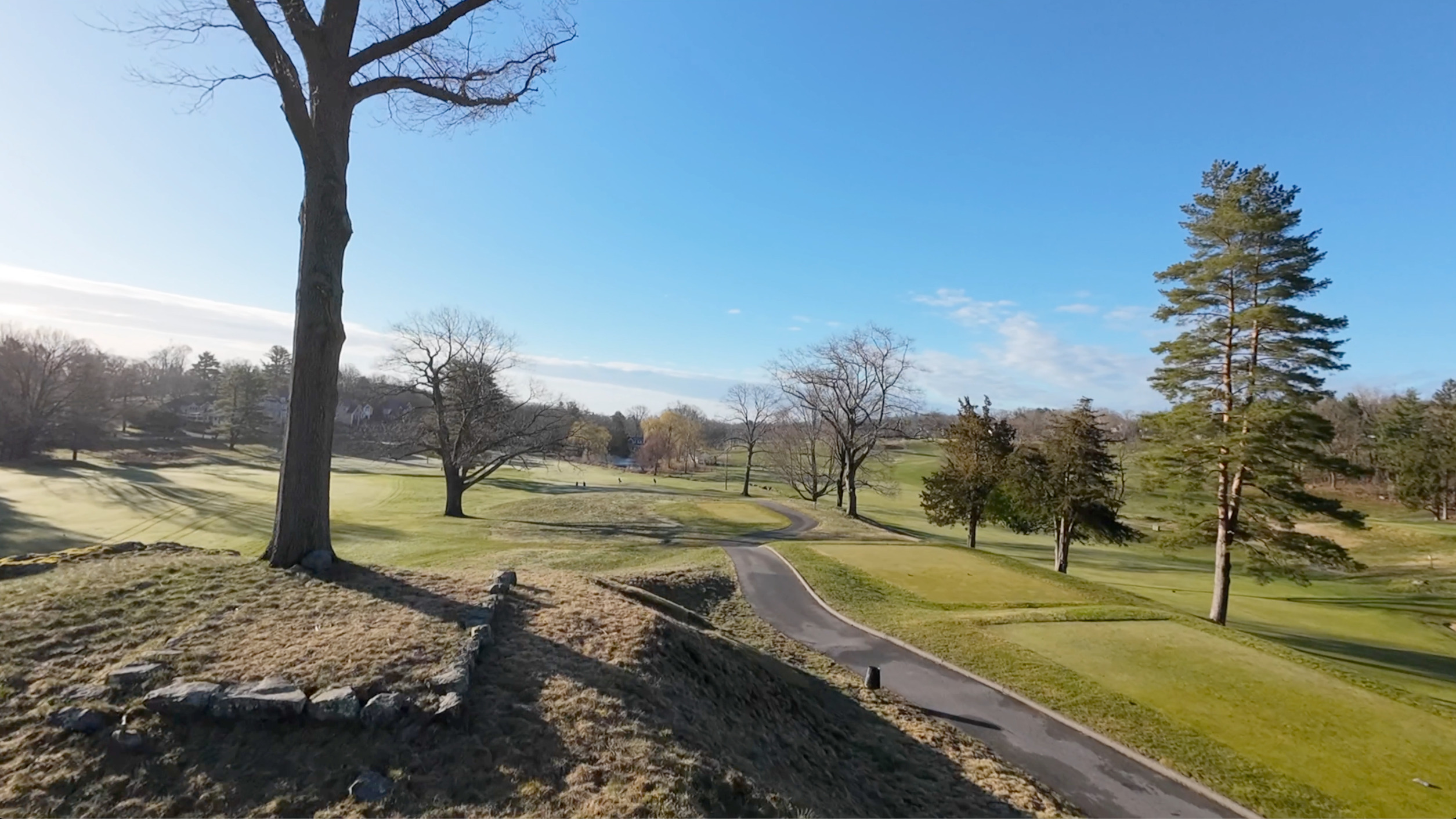
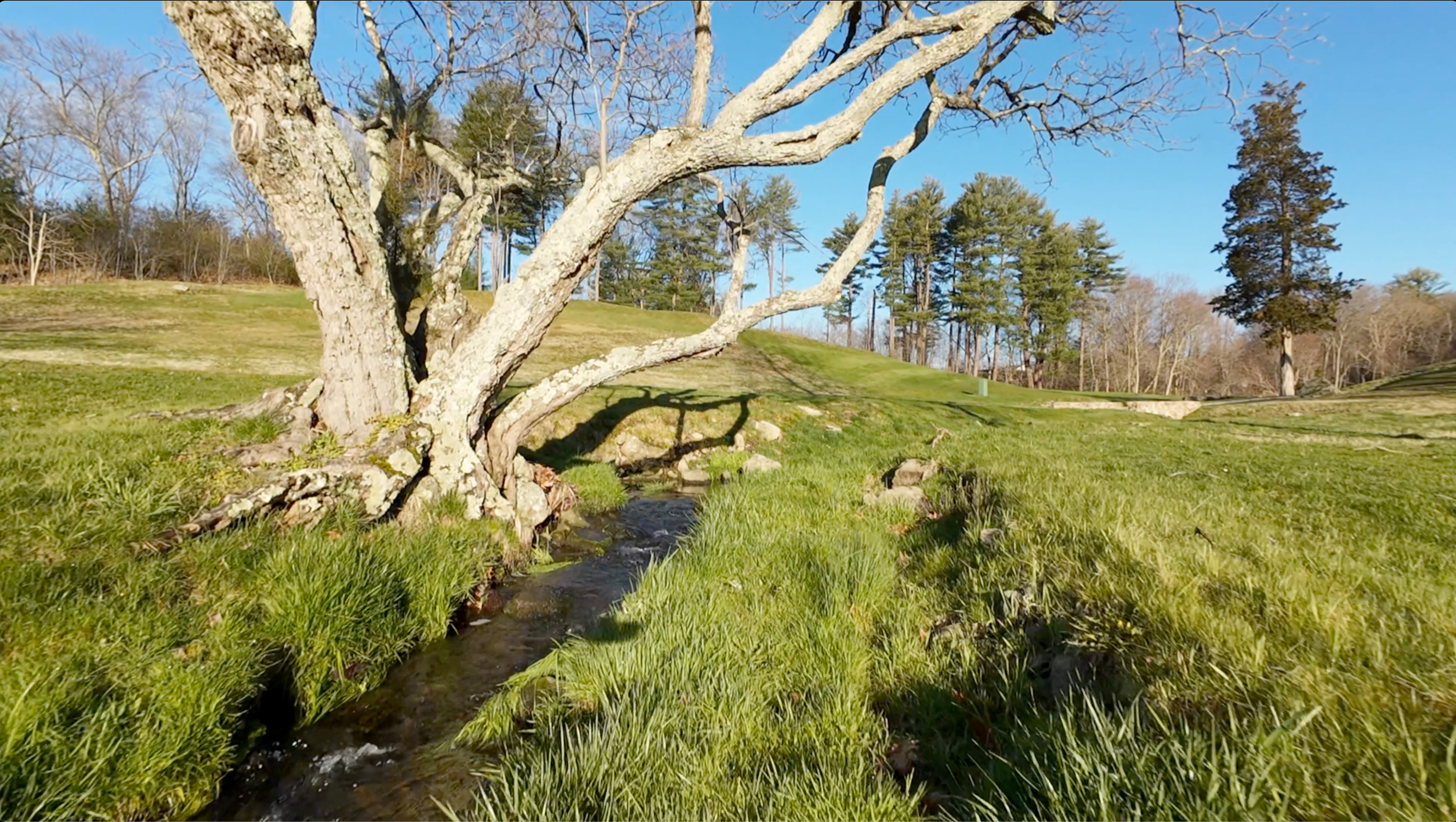
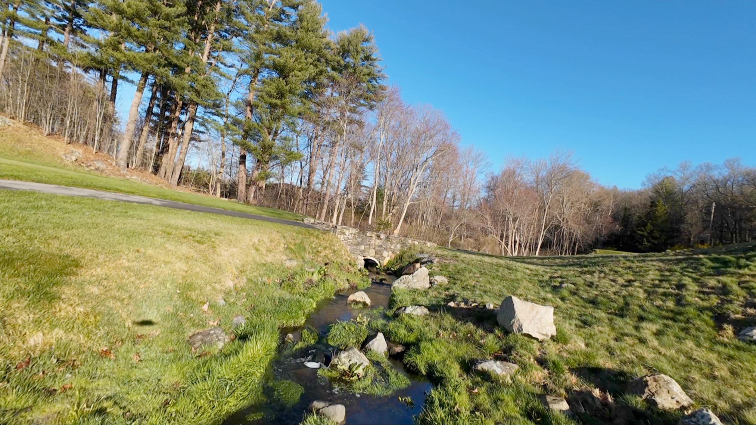
Here are some screenshots from this recording. The pictures were shot with the new Avata 2, a more advanced camera than the old Avata (which I still have). I recorded first in Winchester on the golf course and then on the Shannon beach. During the recording the weather quickly changed from sunny to covered.