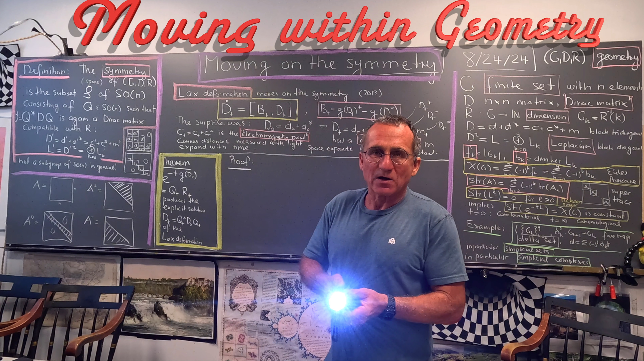
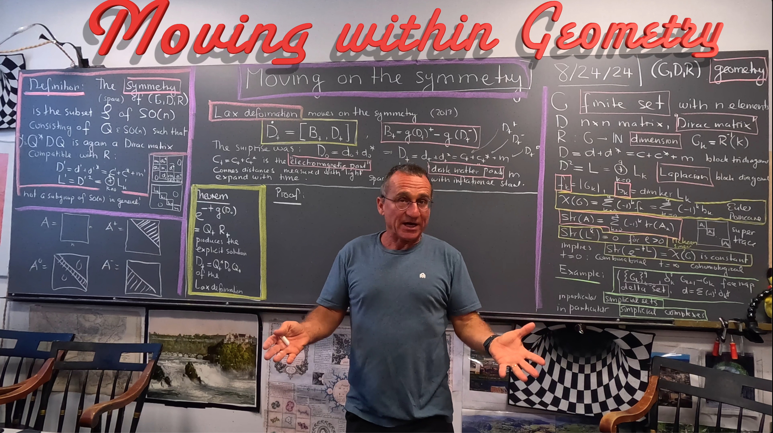
Here is the proof that is solved by
with
, the QR decomposition. Proof. We show that
is solved
. From
by $Q_t$ with
, we get
. Look at the differential equations
for Q,R with initial condition
. The first equation gives the conjugating orthogonal transformation. Then,
. But we also have
. Comparing this gives
. Since
is invertible this means
or
which follows from
. This connection verifies the “dark matter lemma” which I mentioned 2 weeks ago (but gave a defective proof): the QR decomposition flow preserves Dirac matrices. It is not obvious at all at first that
is block tri-diagonal, even if
are. The matrix
is not in the algebra generated by
or
which can be seen from the fact that
is not block tridiagonal. Also, the algebra generated by
changes with time. Different
do not commute in general. Also, the curve of matrices
is not a translation on
, it moves on a geodesic in the isospectral set although.
Update: Here is the write-up for this note. [PDF] (and on the ArXiv) It is a remark of course but very exciting for me as I did not expect the QR story to over to this geometry set-up (I have in the last 10 years not even tried because I thought it would be too far fetched). For me, it is a fundamental insight that we can look at relatively large symmetry sets of rather finite geometries and have time evolutions that produce interesting dynamics. No initial conditions are needed besides the geometry. Discrete mathematics in general suffers from the lack of continuum symmetries. If we look at the automorphism group for example, the this is in general trivial. Most networks or manifolds do not admit any discrete symmetry at all, completely opposite to what we see in the continuum, where the diffeomorphism group is a rich and huge infinite dimensional group. This lack of symmetry in a discrete setting really hurts. But in the quantum world (meaning when looking at operator algebras related to the Dirac matrix defining the geometry), there is lots of symmetry. Given the almost too obvious fact that symmetry is so essential in all the physics we know (physics essentially is the story of symmetries), this is a huge relieve.
Here is the Mathematica code. As usual, I try to keep things as compact (simplicity!) as possible, doing things in one line if possible. Like the Runge-Kutta procedure RK which makes the numerical solution of the ODE more transparent. Mathematica has built in NDSolve routine,s but it is not clear what such implementations actually do under the hood and doing it with NDSolve would make the code even larger. The following code of course contains more than we really need and almost half of it is just formatting so that the Dirac matrix can be plotted in the right Block -Jacobi -Form. We had built the Dirac routines about 12 years ago and had then opted to implement the dimension function R in integrated form. For an octahedron for example (CompleteGraph[{2,2,2}]] we have the integrated dimension vector b=(0,6,18,26) rather than the dimension function R=(6,12,8) for the geometry (G,D,R). As mentioned at various places and also in the talk below, if we have a simplicial complex or start with a finite simple graph, then (G,D,R) are canonically given. But for a delta set, like an open set given by a level surface or co-dimension k manifold in a d-manifold, the dimension function is required as the smallest dimensional “points” are simplices of positive dimension in the Sard story (the theme of last fall, winter and spring) or the finite topology setting, where open sets need also a dimension function (the theme from 2 years ago). In the octahedron case, where G contains 26 sets and one of them is the face x={1,3,6}, then is an open set. As a delta set, it looks like a point, because G has just one element and there is nothing else there. But the dimension of this point is R(x)=2. The object (U,D,R) is a geometric object with cohomology (Betti vector (0,0,1)). Keeping track of dimension is also needed when we look at Cartesian products as the smallest dimensional points like (1,2) are assigned zero dimension. Doing all this in the frame work of delta sets is awkward and we opted early to do things in a computer science point of view way: what is important are the data structure which can be implemented fast and in a poetic way, not the mathematical beauty (presheave), where the set-up is poetic (a functor category) but the implementation is ugly. What counts for me is how elegantly one can implement the structure in full detail and work with it. Simplicity, Clarity and Generality usually go well together. The data structure approach is even much more general than the more abstract pre-sheaf setup, where the exterior derivative is directly tied to the face maps. [Upate August 27, 2024: since mathematica does sometimes get different signs in the diagonal of R (unlike what the theory demands, we rectify this here. Before we just had “corrected” corrected that by ignoring the last row and column].
Generate[A_]:=If[A=={},{},Sort[Delete[Union[Sort[Flatten[Map[Subsets,A],1]]],1]]];
Whitney[s_]:=Union[Sort[Map[Sort,Generate[FindClique[s,Infinity,All]]]]]; L=Length;
sig[x_]:=Signature[x];   nu[A_]:=If[A=={},0,L[A]-MatrixRank[A]];  omega[x_]:=(-1)^(L[x]-1);
F[G_]:=Module[{l=Map[L,G]},If[G=={},{},Table[Sum[If[l[[j]]==k,1,0],{j,L[l]}],{k,Max[l]}]]];
sig[x_,y_]:=If[SubsetQ[x,y]&&(L[x]==L[y]+1),sig[Prepend[y,Complement[x,y][[1]]]]*sig[x],0];
Dirac[G_]:=Module[{f=F[G],b,d,n=L[G]},b=Prepend[Table[Sum[f[[l]],{l,k}],{k,L[f]}],0];
   d=Table[sig[G[[i]],G[[j]]],{i,n},{j,n}];{d+Transpose[d],b}];
Hodge[G_]:=Module[{Q,b,H},  {Q,b}=Dirac[G];  H=Q.Q;
   Table[Table[H[[b[[k]]+i,b[[k]]+j]],{i,b[[k+1]]-b[[k]]},{j,b[[k+1]]-b[[k]]}],{k,L[b]-1}]];
Betti[s_]:=Module[{G},If[GraphQ[s],G=Whitney[s],G=s];Map[nu,Hodge[G]]];
Fvector[A_]:=Delete[BinCounts[Map[L,A]],1];    Euler[A_]:=Sum[omega[A[[k]]],{k,L[A]}];
 QRDeformation[B_,t_]:=Module[{Q,R,EE},{Q,R}=QRDecomposition[MatrixExp[-t*B]];
     EE=DiagonalMatrix[Table[Sign[R[[k,k]]],{k,Length[R]}]]; Q=EE.Q; R=R.EE; Q.B.Transpose[Q]];
DiracPlot[{B_,b_}]:=Module[{S1,S2,S3},n=L[B];S1=MatrixPlot[B,FrameTicks->None,Frame->False];
S2=Graphics[{Thickness[0.001],Table[Line[{{0,n-b[[k]]},{n,n-b[[k]]}}],{k,L[b]}]}];
S3=Graphics[{Thickness[0.001],Table[Line[{{b[[k]],0},{b[[k]],n}}],{k,L[b]}]}];Show[{S1,S2,S3}]];
LowerT[A_]:=Table[If[i>=j,0,A[[i,j]]],{i,Length[A]},{j,Length[A[[1]]]}];
Str[B_,b_]:=Module[{},Sum[-(-1)^k*Sum[B[[b[[k]]+l,b[[k]]+l]],{l,b[[k+1]]-b[[k]]}],{k,L[b]-1}]];
RK[f_,x_,s_]:=Module[{u,v,w,q},u=s*f[x];v=s*f[x+u/2];w=s*f[x+v/2];q=s*f[x+w];x+(u+2v+2w+q)/6];
DiracDeformation[DD_,tt_]:=Module[{dt=1./10^5,d,e,B,dd=DD,TT}, NN=Floor[tt/dt];
   Do[d=LowerT[dd];e=Transpose[d];B=e-d;FF[x_]:=B.x-x.B;dd=RK[FF,1.*dd,dt],{NN}];dd];

s=RandomGraph[{8,20}]; G=Whitney[s];{B,b}=Simplify[Dirac[G]]; n=Length[B];
V[X_]:=Max[Abs[Flatten[Table[X[[k,l]],{k,n},{l,n}]]]];
B2=DiracDeformation[B,0.12]; B1=QRDeformation[B,0.12]; Print["Difference: ",V[B2-B1]];
Print["Supertracetests= ",{Str[B2.B2.B2.B2,b], Str[MatrixExp[-1.0*B1.B1],b]}]
S=GraphicsGrid[{{DiracPlot[{Chop[B],b}],DiracPlot[{Chop[B1],b}]}}]


