Connected Sum - Quantum Calculus

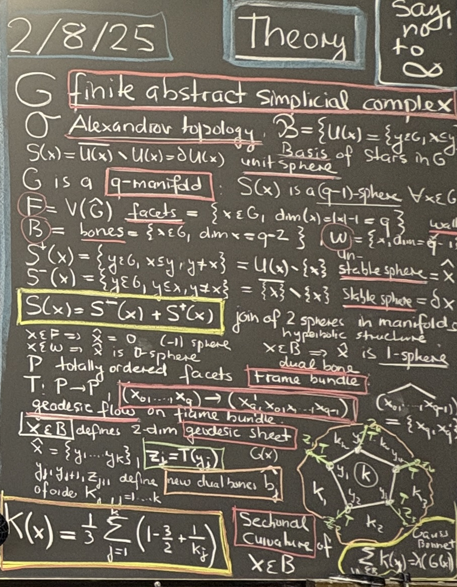
There is a typo in the K(x) formula. It should be [sum (1-k/2+2/kj)]/3

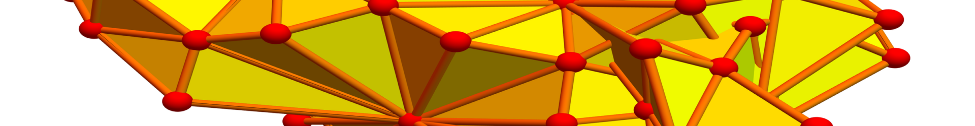
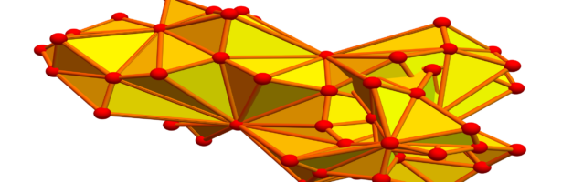
We continue to look at examples of a-manifolds. Besides level sets we can also do connected sum constructions. In the talk, I glue together two manifolds along a q-simplex. An other possibility is to glue along a wall, a (q-1) simplex, removing two simplices attached at a hypersimplex and glue together. A bit more restrictive is to glue along a (q-1) simplex x as we need now the dual simplex $\hat{x}$ which is always a circle, to have the same length. In general, we can take in each manifold a k-simplex x and y and glue along them as long as the dual $\hat{x} = \bigcap_{v \in x} S^+(\{v\})$ are isomorphic. Note that this works also for non-manifolds! I mention the important hyperbolicity $S(x) = S^-(x) + S^+(x)$ which holds for all simplicial complexes $G$ and all simplices $x \in G$ . I made already heavy use of this in 2016 (see this talk from October 2017). Manifolds can be characterized by the fact that the stable sphere $S^+(x) = U(x) \setminus \{x\}$ (an open set in the Alexandrov topology is also a sphere (in the sense that its Barycentric refinement (which is a simplicial complex) is a sphere). The identity $S(x) = S^-(x) + S^+(x)$ is then an identity in the sphere submonoid of the Zykov monoid in which the join is the addition. As maybe exaggerated a bit in the talk: the setup is really simple. The geometric structure of a finite abstract simplicial complex has one axiom only: it is a finite set of non-empty sets closed under the operating of taking finite non-empty subsets. The topology on G is generated by the stars $U(x) = \{ y, x \subset y\}$ . The notion of sphere is inductive in that G is a manifold with the property that there exists $x \in G$ , such that $G \setminus U(x)$ (which is a simplicial complex as it is a closed set obtained by taking away an open set from a closed set) is contractible. Contractibility is also defined inductively. G is contractible if there exists an x such that $S(x)$ and $G \setminus U(x)$ are both contractible. All this is more elegant than when formulating it within graphs. It can be more intuitive however to use graphs. See lecture 10 [PDF] and lecture 18 [PDF] in this differential geometry course. Simplicial complexes are slightly more general and can be useful, especially if one wants to work with very small structures as Whitney complexes of graphs are in general larger. As hinted in lecture 10 mentioned above, the concept of connected sum is also useful to get an intuitive notion of what it means to be homeomorphic. Two manifolds can be considered homemorphic if one get from one to the other by a finite sequence of connected sum operations, where the second is a q-sphere. Gluing in a q-sphere or removing a q-sphere (as long as the result remains a manifold) does not change the topological type of the manifold. Higher characteristics or higher cohomology or analytic torsion really need topological equivalence. Not like simplicial cohomology which is much more forgiving and remains intact after homotopy deformations (which can destroy the manifold property).

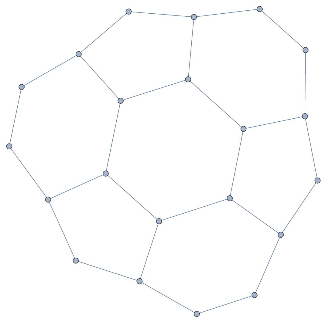
A geodesic sheet is defined in arbitrary manifolds, whatever the dimension is. It gives a notion of sectional curvature. can be seen as a flower, where the central bone is the whorl and the attached dual bones are the petals. The size of these polygons determines the curvature of the original bone (co-dimension 2 simplex) in the simplicial complex. The resulting curvature satisfies Gauss-Bonnet and gives a good sectional curvature notion much better than just taking the central bone size which does not involve the geodesic flow at all. Regge calculus only considers this. It is too rigid however when trying to define sectional curvature which has a chance to produce the classical positive curvature manifolds.

What is new since this winter is that we have a general geodesic flow for a q-manifold. It is canonically defined and does not need an additional structure like a connection. It defines a connection. This is good as also in the continuum, we have by the fundamental theorem of differential geometry a unique torsion free connection compatible with a metric. Now, here it is given by the simplicial complex alone and also defines a notion of distance. It needs however a manifold structure as it is crucial that every (q-1) simplex x (called “wall“) has a 0-sphere $\hat{x} = \{a,b\} \sim S^+(x)$ as a stable sphere. Now the geodesic flow is defined as the map $T( (a,x_1,x_2,\dots,x_{q}) = (x_1,x_2, \dots, x_q,b)$ . This depends on the total order defined on the simplex and so is a map from the frame bundle P onto itself. The frame bundle is the set of totally ordered maximal simplices. As for sectional curvature, we need a notion of 2-dimensional direction (which in the continuum is a 2-dimensional plane in the tangent space). We do that by looking at a (q-2) simplex x (called “bone“). This nomenclature has been used in Regge frame works, where it is used to define the discrete Hilbert action. In a 4-manifold it is a triangle. Note however that Regge used Euclidean notions like excess angles from the continuum. Regge therefore is a numerical scheme approximating notions from classical differential geometry which uses the Euclidean stuff. ( I tried at least for some time to be a mathematical physicist … but mathematical physics is too hard and too close to engineering, where one can always argue whether a scheme is a good model. In pure mathematics, one at least try to be a poet and look for the most elegant approach, and not be interested at first whether it produces a good numerical scheme. By the way, the discrete frame work so far behaves actually quite well. For me the eventual measuring stick is whether one can prove results like whether positive curvature implies positive Euler characteristic for even dimensional manifolds. I have not found a counter example in the discrete so far but also did not search widely. ln order to search one has to have a lot of manifolds to test with and the connected sum construction is one of the elegant constructions to build new manifolds from old ones. ). The manifold property immediately implies that the dual $S^+(x) = \hat{x}$ of such a bone is a one-dimensional sphere, a circle. Now, lets assume that $(y_1,\dots,y_k)$ is such a circle (it consists of all maximal simplices which contain the bone x. In the 2 dimensional case for example it consists of all triangles which contain a given vertex x). Having a bone, we can now use the geodesic flow to extend the bone to a geodesic sheet which then will be used to compute curvature. Of course, the orientation of the bone matters! Choosing a total order on a simplex is like introducing a “basis” on it. The first element $x_0$ is the “zero” and the other points $x_k$ define “basis vectors” $(x_0,x_k)$ . Now, given a bone $x=(x_0,x_1,\dots, x_{q-2})$ a point in the dual bone has the form $y_k=latex (x_0,x_1,\dots,x_{q-2},u,v)$. Now, if we apply the geodesic flow to such a point, we get a point $T(y_k) = z_k$ which is of the form $(x_1,x_2, \dots, x_{q-2},u,x_o')$ , where the dual of $(x_1,\dots,x_{q-1},u)$ is a 0-dimensional sphere which means two isolated points (x0,x0′) , which corresponds to the two maximal simplices attached to the wall, note that any union of maximal simplices by definition is an open set that is topologically 0-dimensional in that its Barycentric refinement is zero dimensional). Important is now also the fact that any path graph of length 2 in the dual graph $\hat{G}$ (where vertices are maximal simplices and connections are done if they intersect in a wall) define a unique bone. (You could call this the bone lemma. It is analog that the intersection of the two maximal simplices $x,y$ in an edge $(x,y) \in E(\hat{G})$ form a wall $x \cap y$ .) The bone lemma tells that if (a,b),(b,c) are edges in the dual graph $\hat{G}$ then $a \cap b \cap c$ is a bone. Now, this gives us a nice structure of the geodesic sheet. It has a nice flower structure: there is a central dual bone = whorl surrounded by secondary dual bones = petals. This structure now defines sectional curvature. First of all, we can for every maximal simplex $y = y_k$ in the dual bone define the form curvature which in the 2-dimensional case is the Ishida-Higushi curvature. The idea of k-form curvature is natural: just distribute the “energy” $w(x)$ of any simplex and distribute it to the k-dimensional simplices. In the 2-dimensional (Ishida-Higushi) case, where we look at the dual graph and attach a curvature to the vertices by taking the energy of the vertex 1, subtract 3/2 because the vertex degree is 3 and each vertex distributes half to each of its two ends, then add the sum of $1/k_j$ where $k_j$ is the polygon size. So the form energy of one of the vertices is $K(y_j) = 1-3/2 + 1/k_a + 1/k_b+1/k_c)$ . Now add up all these curvatures over all the $y_j$ in the whorl=dual bone of the flower. What happens if we add up all these curvatures $1/k_j$ we get three dimes the contribution (I think now that the formula on the board is not correct as stated. It should be $K=[1-k/2+\sum_j 2/k_j]/3$ . This is a good second order curvature also for triangulated 2-manifolds. It averages quantities involving the vertex degrees of the unit ball. We could not just average the Eberhard curvature 1-deg(x)/6 over a ball. That would be numerical scheme but not satisfy Gauss-Bonnet. I had been looking for a second order curvature since 2010 (see this article from 2012). Now we have $(1+deg(x)/2 + \sum_{y \in S(x)} 2/deg(y))/3$ . This sums up Ishida-Higushi curvatures of the triangles attached but then makes an additional step and moves these curvatures back to the vertex. The Ishida-Higushi curvature applied directly to a triangulated 2-manifold is identical to the Eberhard curvature 1-deg(x)/6 which has been known more maybe 150 years ago and became popular 100 years ago in the context of graph coloring, especially with Birkhoff and Heesch.

Author: oliverknill