Second Order Poincare-Hopf - Quantum Calculus

Shortly after working on Gauss-Bonnet-Chern for graphs, I wrote about Poincare-Hopf for graphs. It took a larger part of the winter break 2011/2012 to come up with the formula $i_f(v) = 1-\chi(S_f^-(v))$ where $S_f^-(v)$ is part of the unit sphere $S(v)$ where the function value is smaller than the function value at v. The function f is assumed to be a coloring which implies that the vfunction values on $S(v)$ are all different from $f(v)$ . The proof given there in 2011 is a bit convoluted. It occurred to me only later that the statement is almost tautological if one thinks about $\omega(x) = (-1)^{{\rm dim}(v)}$ as an energy and $\chi(G) = \sum_{x \in G} \omega(x)$ as the Euler characteristic. Poincare-Hopf is then obtained by shoving all energies $\omega(x)$ to the vertex $v \in x$ where $f$ is minimal.

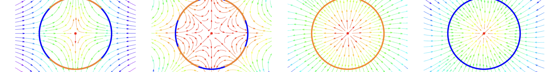
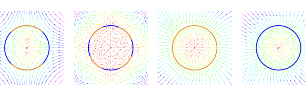
It is quite amazing how “expensive” in comparison the Poincare-Hopf statement in the continuum is. The most elegant formulation sees it as the degree of the sphere map $T$ from a small sphere $S_r(v)$ to the unit sphere defined by $T(v) = F(v)/|F(v)|$ . This is a topological notion which can be defined without smoothness assumption but it can be computed using calculus. In the discrete of course, we don’t have any linear algebra nor smoothness at our disposal. But the discrete setting is completely equivalent at least if the vector field is a gradient field $F=\nabla f$ and $f$ is Morse. In that case the Euler characteristic of $S_f^-(v)$ is either $0$ or $2$ depending on whether the stable sphere is even or odd dimensional. The stable sphere is the intersection of the stable manifold at the critical point with the small sphere $S_r$ .

Poincare-Hopf is pivotal for many reasons. First of all, it is really nice to have divisors rather than smooth curvature functions. Maybe nature takes this point of view when looking at “particles” rather than “fields”. There is practical value because if we have a clever function $f$ , we can easily compute the Euler characteristic of the manifold. This is especially useful for large dimensional manifolds. Maye the most important reason is that Poincare-Hopf is the connection between the continuum and the discrete. It is much easier to link the divisors in the discrete and continuum case than to link the curvature, in particular because the Riemann curvature tensor is a mess in the continuum (in comparison).

In this video, I push the idea a bit further and show that also higher order curvature formulas have an index expectation interpretation. (all obvious once you see it). The simplicity of the set-up of course also produces prejudice. Both of my articles from 2011 and 2012 never got a referee report. It was not even worth looking at it! It had been sent to a graph theory journal. I attribute the arrogance today also to the fact that there was (at least then in 2011) a cultural issue: graphs were proudly touted (and are still in most graph theory books) as one dimensional simplicial complex. But the discrete curvature is completely in line with the continuum even so the continuum is so much more restrictive. Both Gauss-Bonnet and Poincare Hopf work for arbitrary graphs, for arbitray simplicial complexes and even in the topos of delta sets. Manifolds of course work too but they are only a very special case. In the continuum, curvature only is set-up for even dimensional manifolds (at least if curvature is understood as an intrinsic curvature that satisfies Gauss-Bonnet). The theme of Gauss-Bonnet (as I talked and wrote about extensively over the last 15 years now) can be extended to so much larger frame works, some of which do not even exist in the continuum, like higher characteristics or ring valued energized complexes. It is the simplicity which makes the frame work quite flexible: Poincare-Hopf pushes the energies of the energies of space deterministically to the zero dimensional part of space, while Gauss-Bonnet does it in a random way. Curvature therefore is always index expectation. It produces also almost tautological proofs that curvature of odd dimensional manifolds is contant 0, simply because symmetric indices can be written as an Euler characteristic of a $q-2$ dimensional manifold (a submanifold of the unit sphere). And as odd dimensional manifolds have zero curvature they have zero dimensional Euler characteristic.

Here is some code computing the second order Poincare-Hopf indices. Note that we need that the highest dimensional facets cover the graph or the simplicial complex. The reason is that we shove first the energies to the facets. If there is no facet for part of the graph, these energies are lost. That of course works for manifolds, which are pure simplicial complexes.

Generate[A_]:=If[A=={},{},Sort[Delete[Union[Sort[Flatten[Map[Subsets,A],1]]],1]]];
Whitney[s_]:=Generate[FindClique[s,Infinity,All]]; w[x_]:=-(-1)^Length[x];
Euler[s_]:=Total[Map[w,Whitney[s]]];

Index[s_]:=Module[{G0=Whitney[s],G1,G3,F1,F2,W0,W1,W2,q},q=Max[Map[Length,G0]];
G1=Select[G0,Length[#]==1&];G3=Select[G0,Length[#]==q&];
F1=Table[G0[[k]]->RandomChoice[Select[G3,SubsetQ[#,G0[[k]]] &]],{k,Length[G0]}];
F2=Table[G3[[k]]->RandomChoice[Select[G1,SubsetQ[G0[[k]],#] &]],{k,Length[G3]}];
W0=Table[-(-1)^Length[G0[[k]]],{k,Length[G0]}]; W1=W2=Table[0,{Length[G0]}];
Do[x=G0[[k]];W1[[Position[G0,x /.F1][[1,1]]]]+=W0[[k]],{k,Length[G0]}];
Do[x=G0[[k]];W2[[Position[G0,x /.F2][[1,1]]]]+=W1[[k]],{k,Length[G0]}];
Table[W2[[k]],{k,Length[G1]}]];

s=CompleteGraph[{2,2,2,2,2}];
i=Index[s]; Print[i]
{Total[i],Euler[s]}

March 5 addendum: And here is some code which illustrates the gradient case. This is more relevant for linking the discrete with the continuum. The set up is that we have a function on facets of a manifold as well as a function on vertices of the manifold. Now first use the function on facets to distribute all energies of simplices to the facets: just move every simplex energy to the facet surrounding it on which the function is minimal. Then in a second stage, move all the energies from the facets to the vertices. The end effect is the same than as for the usual Poincare-Hopf which directly moves everything to the vertices, but there is a big difference. It is a second order notion and simplices not containing a given vertex can still contribute. It has two effects, first of all the range of the indices can become bigger. So, after index expectation, also the curvature can become more substantial. But it also produces the curvature we had explored before and it just makes much more sense in examples. Remember, we want to have a good notion of sectional curvature that reflects the continuum notion well. A first order curvature does not make sense at all as the Mickey-Mouse theorem illustrates. There we had asked that every embedded wheel graph has positive curvature, a very very rigid notion forcing all positive curvature manifolds to be tiny of diameter 2 or 3 and being spheres. What we want is to have the known spectrum of positive curvature manifolds. The remark of this talk was just that also for second order curvatures we have an index expectation and so the possibility to tune the weights. But like in LLM’s having more weights to play with makes things also more powerful. We do not want to produce a third order curvature (evenso this is no problem to make, just repeat the process), and the reason is simple: we not only want a power notion of curvature, we want it also to be simple enough that we can prove things. We are mathematicians after all and not engineers. Engineers are less interested in proofs.

Generate[A_]:=If[A=={},{},Sort[Delete[Union[Sort[Flatten[Map[Subsets,A],1]]],1]]];
Whitney[s_]:=Generate[FindClique[s,Infinity,All]]; w[x_]:=-(-1)^Length[x];
ToGraph[G_]:=UndirectedGraph[n=Length[G];Graph[Range[n],
  Select[Flatten[Table[k->l,{k,n},{l,k+1,n}],1],(SubsetQ[G[[#[[2]]]],G[[#[[1]]]]])&]]];
Barycentric[s_]:=ToGraph[Whitney[s]]; Euler[s_]:=Total[Map[w,Whitney[s]]];

Index[s_]:=Module[{G,V,F,(* f,g,*)W,J,q}, (* constructs index with functions on vertices/facets*)
G=Whitney[s]; q=Max[Map[Length,G]]; (* clique number = dim(G)+1 *)
V=Flatten[Select[G,Length[#]==1&]]; (*vertices*) F=Select[G,Length[#]==q&];  (* facets *)
f=Table[V[[k]]->Random[],{k,Length[V]}]; g=Table[F[[k]]->Random[],{k,Length[F]}];
minf[x_]:=x[[First[Flatten[Position[x /. f,Min[x /. f]]]]]]; (* the minimum position of f on x *)
ming[x_]:=Module[{S=Select[F,SubsetQ[#,x] &]},S[[First[Flatten[Position[S/.g,Min[S/.g]]]]]]];
W=Table[G[[k]] -> -(-1)^Length[G[[k]]],{k,Length[G]}];   (* primordial energy *)
J=Table[0,{Length[V]}]; Do[x=G[[k]];J[[minf[ming[x]]]] += (x /. W) ,{k,Length[G]}]; J]

s=Barycentric[PolyhedronData["Icosahedron","Skeleton"]];i=Index[s]; Print[{i,Total[i],Euler[s]}];
s=Barycentric[CompleteGraph[{2,2,2}]]; i=Index[s]; Print[{i,Total[i],Euler[s]}];

Author: oliverknill