Curvature for Partitions - Quantum Calculus

A discrete 2-manifold [PDF] is a finite simple graph for which all unit spheres $S(v)$ have d(v)=4 or more vertices. The smallest example is $K_{2,2,2}$ which is the octahedron graph and where every unit sphere is a circular graph with 4 elements. The Eberhard curvature $K(v) = 1-d(v)/6$ is very rigid: the Mickey Mouse theorem tells that every positive curvature manifold must be a sphere. This result even extended to d-manifolds for which every embedded wheel graph has positive curvature at the center. One remedy is to allow curvature to be more flexible like having $K(v) = E[i_f(v)]$ where $i_f(v)=1-\chi(S^-_f(v)$ is the Poincare-Hopf index of a function and $E$ is the expectation for a probability space $(\Omega,\mathcal{A},P)$ of locally injective functions on the vertices of the graph. This index expectation is also the link which connects the continuum with the discrete. In full generality the Levitt curvature $K(v) =\sum_{k=-1}^{\infty} f_k(S(v))/(k+2)$ (with $f_k(G)$ measuring the number of k-simplices in G with $f_{-1}=1$ , then this is the index expectation where the probability measure is the uniform distribution of IID random variables on the vertices or the finite probability space of all graph colorings with some color. The probability space can be deformed and links directly to the Gauss-Bonnet-Chern curvature because also the later can be seen as an index expectation, where the 2n-manifold is embedded in a large dimensional Euclidean space which defines a nice rotational symmetric probability measure on all Morse functions that come from linear functions in the ambient space. If the graph is a triangulation of that manifold then the indices align and the index expectation naturally converts to the classical measure which is a Pfaffian of the Riemann tensor.

Since the two dimensional naive Eberhard curvature does not work as a sectional curvature (as positive curvature implies sphere which is unacceptable) we needed a better notion of sectional curvature. As the continuum suggests, this is related to define a natural geodesic flow but also here there are difficulties if one takes paths on edges. The solution pursued last winter was to look at paths on maximal simplices and look at a total order on a simplex as a notion of frame so that if all maximal simplices are ordered, we get a frame bundle. This is also not new. I had looked at total orders on simplices before to have a notion of vector field on a graph. See this paper from 2019. The idea was that a Poincare-Hopf index is defined if we can on any simplex x get a vertex $F(x) \in V$ . This is the vertex onto which the energy $\omega(x) = (-1)^{{\rm dim}(x)}$ is mapped to. Doing this assignment deterministically produces an integer index, that is a divisor. Curvature is obtained by distributing the curvature according to weights of a probability space. Poincare-Hopf can also be seen as an index expectation, and the indices can be seen as curvatures too.

The good definition of geodesic flow was now $T(x_0,x_1 ,\dots,x_n) = (x_1,\dots,x_n,y_0)$ , where $y_0$ is the point dual to $x_0$ in that the dual simplex $(x_0,y_0)$ of the (q-1)- simplex $(x_1,\dots, x_n)$ . Every k-simplex $x$ in G naturally has a dual simplex $\hat{x}$ which is the intersection of all unit spheres of vertices in x. In the case of a q-manifold, the dual of a k-simplex is a (q-k-1)-sphere. The dual of a vertex is the unit sphere $S(v)$ . The dual of a $(q-1)$ simplex (a “wall”) is a 0-sphere which are two isolate points like $(x_0,y_0)$ used in the definition of geodesic flow. For defining sectional curvature, we have to look at 2 dimensional notions and so at $(q-2)$ simplices (“bones”) for which the dual is a circle of size m. This is the circle which is considered in Regge calculus from the 1970ies but Regge calculus looks at discrete stuff embedded in a given manifold which is just a numerical scheme. We prefer not to take an ambient space for granted but stay in the discrete. That is not only categorically honest (in combinatorics, we should not refer to the continuum) but also shields us from a disaster like that the axiom system of ZF turns out to be inconsistent. (In the TV series “fallout” from last year, the event of a nuclear catastrophe is well displayed. We can not exclude this to happen to humanity, we can also never prove (as Goedel showed) that the axiom system ZF is consistent. So it is nice to have shelters to retreat to and finite mathematics is a nice shelter.

Now, when we defined sectional curvature we took the dual sphere of a bone and used the geodesic flow to build adjacent bones, building so a geodesic sheet. The dual of that is part of a 2-manifold. Now, we have taken the form curvature (which in the 2-dimensional case is the Ishida-Higushi curvature but we now take these curvatures on the vertices of the sheet which are triangles in the dual sheet and push it to the vertices. Now, we have a curvature for 2-manifolds that looks a bit more complicated but is very well behaved. The important formula is

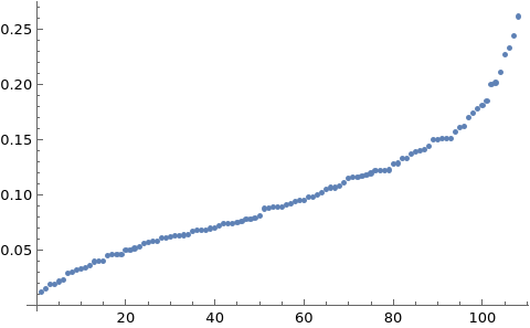
$K(v) = \frac{(2-d(v))}{6} +\frac{2}{3} \sum_{w \in S(v)} \frac{1}{d(w)}$

where $w$ runs over the unit sphere. While taking about this yesterday, I suddenly occurred to me that this now also produces a curvature for arbitrary partitions. The vertex degrees of the unit circle define a partition $(p_1,p_2, \dots, p_m)$ of the number $n=\sum_w d(w)$ . While doing the board work, I wrote a short program which computes this curvature and which allows to make statistics on how the curvatures behave on all partitions of a large number n. Here it is:

PartitionCurvatures[n_]:=Module[{},p=IntegerPartitions[n];
   Table[(2/3) Sum[1/p[[j,k]],{k,Length[p[[j]]]}]+(2-Length[p[[j]]])/6,{j,Length[p]}]];
ListPlot[Sort[PartitionCurvatures[31]]]

I could get to n=102 before the machine runs out of memory. For larger n, curvatures can become negative. Here is an interesting observation:

For all n smaller than 32, all the partition curvatures are positive!

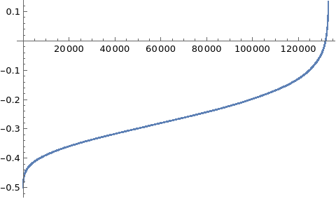
And here is the code when restricting to geometrically meaningful partitions meaning that the number of partitions is larger than 3 and that each entry is larger than 3. I worked on the combinatorics of such cases also in my high school project. Partitions recently came up when looking at level surfaces of manifolds as it produces richer ways to get level sets. Now, most partitions produce negative curvature if n is larger and if restrict to geometric partitions meaning entries larger than 3 and number of entries larger than 3:

PartitionCurvatures[n_]:=Module[{},p=Select[IntegerPartitions[n],(Min[#]>3&&Length[#]>3)&];
   Table[(2/3) Sum[1/p[[j,k]],{k,Length[p[[j]]]}]+(2-Length[p[[j]]])/6,{j,Length[p]}]];
ListPlot[Sort[PartitionCurvatures[80]]]

One could think that for large enough n all curvatures are negative but this is not the case. Here is an example which also shows that we can get arbitrarily small positive curvature values:

K[p_]:=Total[2/(3p)]+(2-Length[p])/6;
K[{4,4,4,4,4,4,4,4,4,4,4,4,4,4,4,4,4,4,4}]   (*gives always 1/3 independent on how many 4 we are adding *) 
K[{5,4,4,4,4,4,4,4,4,4,4,4,4,4,4,4,4,4,4}]   (*gives always 3/10 independent on how many 4 we are adding *) 
K[{6,4,4,4,4,4,4,4,4,4,4,4,4,4,4,4,4,4,4}]   (* gives always 5/18 independent on how many 4 we are adding *)
K[{7,4,4,4,4,4,4,4,4,4,4,4,4,4,4,4,4,4,4}]   (* gives always 11/42 independent on how many 4 we are adding *)
K[{a,b,4,4,4,4,4,4,4,4,4,4,4,4,4,4,4,4,4}]   (* for a>3,b>0 is positive independent on how many 4 we are adding *)
K[{1000000,2000000,4,4,4,4,4,4,4,4,4,4,4,4,4,4,4,4,4}]   (* gives 1/1000000 for example  *)

Author: oliverknill