Gauss-Bonnet Panorama

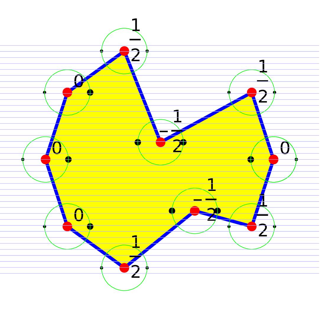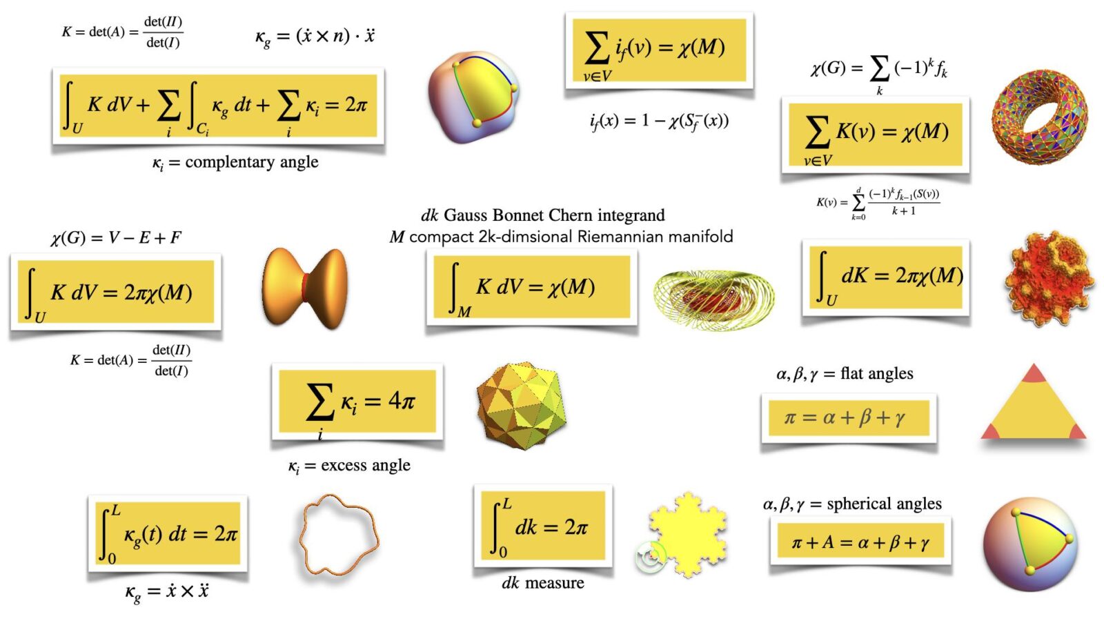
Gauss-Bonnet tells that integrating curvature K over the geometry G is Euler characteristic X. Curvature K is a quantity attached to points in the geometry and Euler characteristic X is an integer. A consequence of the continuity of the functional getting from K to the integral is continuous, a rigidity appears: a deformation of the geometry does not change the Euler characteristic. Something drastic needs to happen, like cutting the geometry appear, or drilling a hole. Gauss-Bonnet works in rather large generality. A piecewise smooth manifold such that the intersections are piecewise smooth manifolds works, any finite simplicial complex, concrete or abstract works, any network works. But as in Riemannian geometry, not only the geometry itself, but an additional structure producing distance matters. The best way is to do this integral geometrically. The reason is that the entire panorama of Gauss-Bonnet collapses to one result. The idea is to have a probability space of functions on the geometry and a notion of “unit sphere” S(v) (which can mean just “very small sphere” in a Riemannian manifold setting) such that S(x) has an Euler characteristic and the level set has an Euler characteristic. This gives an index which is the average of the Poincare-Hopf index for f and -f. What is nice about this index formula (2012) is that it uses only level sets and Euler characteristic of these level sets and that summing up all these indices gives the Euler characteristic of G. Since 2012, the concept of level set has eveolved considerably in the discrete. See this paper for the latest. Curvature is now the expectation of the index over the probability space. The probability space also can serve an other purpose, it also gives a metric on the geometry. For Riemannian manifolds as well as for networks, this produces natural metrics. In the Riemannian case, we can easily get the Riemannian metric from Nash’s theorem. All the examples shown in the panorama work as such, we get the Gauss curvature, the geodesic curvature, the vertex curvature in polyhedral cases, the discrete curvature cases in networks. And it is deformable (which means in fancy modern lingo that we can let machine learning methods run on it, as the probability measure plays the role of the “weights” in learning environments. Lets just illustrate how the simplest case, the school geometry formula or its generalization to simple polygons can be formulated as such. The probability space is the set of unit vectors with the normalized Haar measure on the circle. The index is now, because S(x) is an interval and so has X(S(x))=1, given by which is 0 if one of the two points in S(x) intersected with {f=f(x)} is in the region, which is 1/2 if none is there and -1/2 if both are there. The curvature is exactly the excess angle divided by . The Gauss-Bonnet result obtained by index expectation is equivalent to the old school result that the sum of the angles in a polygon is (n-2) times pi. The picture of the polygon illustrates this. For any Riemannian manifold, place it isometrically into a high enough Euclidean space (possible by Nash’s famous theorem), then use linear maps in the ambient space to produce a curvature. This is the Gauss-Curvature in 2 dimensions and the Gauss-Bonnet-Chern curvature in 2k dimensions. If we take a network with n nodes and place it into space. If the network triangulates a Riemannian manifold and it is geometrically realized, then the index expectation curvature converges to the curvature on the Riemannian manifold. The reason is that also the later can be seen by index expectation.

Here is the youtube presentation