This is a presentation from Saturday, July 13, 2024. Curvatures are usually located on the zero dimensional part of space. I look here at curvature located on one or two dimensional parts of space. In the special case of a triangulation of a 2-dimensional surface, where the usual curvature is K(v) = 1-d(v)/6 with d(v) as the vertex degree, the edge curvature is K( (a,b)) = 1/d(a) + 1/d(b)-1/3 and the face curvature is K((a,b,c)) = 1/d(a) +1/d(b) + 1/d(c)-1/2. They all satisfy the Gauss-Bonnet formula. As I mention in the talk, I’m not so much interested in curvatures that are not based on Gauss-Bonnet and especially not in numerical scheme approximations of classical curvatures. I tried once to define positive curvature manifolds in the discrete assuming that all embedded wheel graphs have positive curvature. This led to the Mickey Mouse Sphere theorem. It was also used as an illustration in my paper “Parameters for Communicating Mathematics”, presented in “a conversation on professional norms in mathematics”. But requiring all wheel sub-graphs to have positive curvature this is a much too strong assumption as all positive curvature manifolds (in dimension 2 or larger) are all spheres. Not even the projective space can be realized as such. I have since tried to soften this like assuming that some index expectation measure induces positive curvature on any wheel graph obtained as intersections of spheres (which is a much weaker assumption but for which I was not yet able to prove the sphere theorem). If the sphere theorem can not be proven with a notion of sectional curvature, it is not the right one. I hope that one can find curvatures which are very local and which do not depend on parts outside a ball of radius 1. An obvious approach is to use Tube type formulas like Herman Weyl did but this leads in the discrete to curvatures for which Gauss-Bonnet fails. I started my work in discrete mathematics with tube like formulas like Puiseux type formulas and looked at the simplest possible Gauss-Bonnet theorem (the Hopf Umlauf satz in the flat plane). This paper from 2010 was my first shot at curvature in the discrete. I rediscovered in that paper also the formula K(v) = 1-d(v)/6 and was very excited until I saw that it is well known (I saw it first in the Princeton companion of mathematics 2009), but we know now it is at least 140 years old and was especially useful for coloring questions: any maximally planar graph must have some vertices of degree smaller 4 or 5, and every maximally planar 3-connected graph is a 2-sphere and so has Euler characteristic 2.
“Kennst du das Land, wo die Zitronen blühn,
Wolfgang Goethe
Im dunkeln Laub die Goldorangen glühn,
Ein sanfter Wind vom blauen Himmel weht,
Die Myrte still und hoch der Lorbeer steht,
Kennst du es wohl?
Dahin! Dahin
Möcht ich mit dir, o mein Geliebter, ziehn!
Kennst du das Haus? auf Säulen ruht sein Dach,
Es glänzt der Saal, es schimmert das Gemach,
Und Marmorbilder stehn und sehn mich an:
Was hat man dir, du armes Kind, getan?”
“What matters
Charles Bukowksi
most
is how well
you walk
through
the fire “
Euler characteristic is the total energy of space. Curvature is what happens if this energy is pushed to points. This can be confusing in the continuum. You just need to read the proof of the Gauss-Bonnet-Chern theorem to see this. Even the simplest proof of Patodi which I learned from Cycon-Froese-Kirsch-Simon’s book as a student is mind boggling. You hardly see any differential geometry course (even on a graduate level) which gives the proof in full detail. The reason for the difficulty is that in the continuum we are blind about lower dimensional parts of space. We need sheaf theoretical crutches to access these parts. We use differential k-forms for example to access k-dimensional parts of space. This requires to build a tensor calculus frame work. This frame work is also needed to take the square root of the Laplacian and are forced to get into Clifford algebras. Spectral questions are obscured by technicalities. We need already some rather heavy functional analysis to tackle elliptic regularity, just establishing that the Laplacian on a Riemannian manifold has discrete spectrum (hardly anything giving much of insight, doesn’t it?) In the talk I made the analogy with Wolfgang Goethe: the more general story of Atiyah-Singer is a bit like high pitched poetry from the 18th century. It is hard to digest. I told in the presentation that in high school, some of my buddies were reading poetry of Charles Bukowksi instead. Goethe is to Bukowski what the Continuum is to the Discrete. The later is more raw, down to earth, brutally simple and feels like blasphemy. The main ideas are present in the discrete however: the analytic index  - dim ker(D^*)")
")
")
 \; {\rm even} \}")
 \; {\rm odd} }")
Last week, I was in my presentation also talking about some challenges I work on. One of the major questions I still have is to get a good notion of sectional curvature. “Good” is not just a feeling. It is quantifiable: the curvature needs to be exact, not an approximation of the curvature we know in the continuum. It should for 2 dimensional surfaces agree with the usual sectional curvature and it should lead to the same theorems as in the continuum. The absolute minimum is to have the Sphere theorem (one quarter pinched positive curvature manifolds are spheres) and the known classification of positive curvature manifolds at least in even dimensions: