We continue the quest to define a sectional curvature for q-manifolds. A good notion should produce classical theorems like that if sufficiently pinched manifolds are spheres. Asking all embedded wheel graphs to have positive curvature was much too rigid and produced only spheres, so small that I called this the Mickey Mouse theorem. We have seen already that for any simplicial complex that is a q manifold there is a good notion of geodesic flow and that there is also a nice notion of geodesic sheet suitable for defining sectional curvature. A sheet is defined by a q-2 dimensional simplex x equipped with a total order. This is analog to the geodesic path which can be seen defined by a q-1 simplex that is totally ordered. The q-2 simplex x defines a dual circle which consists of l facets hinging on the simplex x. For a q=3 manifold for example, where x is an edge, the dual circle consists of all tetrahedra containing x. What we have seen last time is that we can extend the structure naturally by attaching geodesic steps and then use this to build neighboring cycles. we have now a 2 dimensional disk and can attach to each a facet curvature defined in that 2- dimensional disk.
That is a curvature that has been considered by Masashi Ishida (1990, Higushi credits in 1999 Ishida from a workshop on topological graph theory at Yokohama university, Ishida is now at Osaka university) and had been motivated by Gromov’s work, especially the his 1987 paper. Yusuke Higushi (who wrote that paper in 1999) is now at Gakushuin university. It is , where are the lengths of the three faces attached to . This is just the 2-form curvature defined in here (see also the Wolfram entry) in the case of a 2-manifold. Note that this facet curvature for the manifold is a scalar curvature for the dual manifold. If the formula is applied to a triangulated manifold, where each and is the vertex degree, then one gets the usual Levitt curvature which has been considered since Eberhard. Positive Levitt curvature is very restrictive. There are exactly 6 positive curvature 2-manifolds according to the Mickey Mouse Sphere theorem. The reason that I myself had lost track of the Ishida-Higushi curvature (after mentioning it in 2011 in the “Gauss-Bonnet-Chern” for graphs paper) is that for manifolds (meaning simplicial complexes) the notion is the same than the 150 year old notion for a wheel graph. But it also became clear pretty early that the curvature for wheel graphs is a very restricted notion when trying to define sectional curvature. In my Mickey-Mouse paper from 2019, I mention that there are no negative curvature q-manifolds for q>2 for the simple reason that in every q-manifold for q larger than 2 there are lots of triangulated embedded 2-spheres and every 2-sphere must have some positive curvature points (a fact which has been heavily used more than 100 years ago already when investigating the 4-color theorem) because of Gauss-Bonnet and the fact that a 2-sphere has Euler characteristic 2. Taking sectional curvatures as curvatures of embedded wheel graphs is therefore something which will always be confined to the Disney world. it still is an interesting problem in combinatorics. Like how many q-manifolds of positive Mickey-Mouse curvature there are in dimension q. I answered it only for q=2, where there are 6. Going to the facets is not only key for defining geodesic flows but also for defining 2 dimensional geodesic sheets and so sectional curvature. The geodesic sheets are defined as subgraphs of the dual (or better the frame bundle P of . As for defining curvature, we do not have to extend the sheet much and can remain in the dual . But now, the Ishida-Higushi curvature is much better suited. It is a function on the vertices of the dual graph and so a function on the facets of the original q-manifold. What I do then to define sectional curvature for a bone x (a codimension-2 simplex in G), is to sum up these Ishida-Higushi curvatures over every facet that it hinging at the bone x. That triple counts the curvature at every node and if we divide by 3, we get a curvature attached to the bones so that in two dimensions (like for 2-dimensional sheets defined in a q-manifold), we have Gauss-Bonnet on the sheet. That is exactly what happens in the continuum provided we have a geodesic sheet that closes up. Take for example a constant curvature 3-sphere in classical differential geometry. Every geodesic is a circle and every geodesic sheet is a 2-sphere. Since the Euler characteristic of the 3-sphere is zero, there is no way that we can average sectional curvature to get Euler characteristic. The same is true in the discrete.
Example 1) I gave in the talk the example of (the join of two circles) the 4-partite graph defined by the partition (2,2,2,2) which is the smallest 3-sphere and well known as the 16 cell, one of the 6 Platonic polytopes in dimension 3 (some non-topologists look at it as a 4-polytop because it is a triangulation of the 3 sphere embedded in 4-space. This is silly. The 3-sphere also in the discrete is a nice 3-manifold, its facets are tetrahedra, its Euler characteristic is 0, its Betti vector is the Betti vector of the classical 3-sphere). It defines a simplicial complex G with f-vector (8,24,32,16) and Euler characteristic is 8-24+32+16=0. Its Betti vector is (1,0,0,1) like any 3-sphere. It is one of the Mickey Mouse manifolds of positive curvature as every wheel graph that is embedded has 4 elements. The frame bundle has 16*4! = 16*24=384 elements. Every geodesic has length 8. It is a discrete Wiederkehr manifold. Here is an example of one of these periodic orbits of the geodeisc flow {{5, 3, 1, 7}, {3, 1, 7, 6}, {1, 7, 6, 4}, {7, 6, 4, 2}, {6, 4, 2,8}, {4, 2, 8, 5}, {2, 8, 5, 3}, {8, 5, 3, 1}}. This orbit is in the frame bundle P, which is a principle fiber bundle with structure group , where every maximal simplex is ordered. There are only 16 cells {{1, 3, 5, 7}, {1, 3, 5, 8}, {1, 3, 6, 7}, {1, 3, 6, 8}, {1, 4, 5,7}, {1, 4, 5, 8}, {1, 4, 6, 7}, {1, 4, 6, 8}, {2, 3, 5, 7}, {2, 3,5, 8}, {2, 3, 6, 7}, {2, 3, 6, 8}, {2, 4, 5, 7}, {2, 4, 5, 8}, {2,4, 6, 7}, {2, 4, 6, 8}}. Now, every geodesic sheet is a cube. For such a cube, every vertex of the cube is one of the maximal 3-simplices in G and the cube represents a 2-dimensional geodesic sheet. The facet curvature = vertex curvature in the cube is 1-3/2+(1/4+1/4+1/4) = 1/4. Adding this up over all facets hinging at a bone defining the sheet gives 1. Divided by 3 gives the sectional curvature 1/3. This Mickey-Mouse 3-sphere has constant sectional curvature 1/3. Now that is not a good example to sell our story because in this case, also the Wheel curvature (= Eberhard curvature) is constant 1-4/6 = 1/3.
Example 2) Here is a larger 3-sphere, the 49 cell. We take which is the join of two cyclic graphs of length 7. It is a 49 cell because there are 7*7 cells. Now the geodesics can have length 14 or 28. And the sectional curvature are either 1/3 or 4/21. But note that unit spheres are now the suspension of which is a prism graph for which there are points of Eberhard curvature 1-7/6=-1/6. This is no more a “Mickey-Mouse manifold” as some embedded wheel graphs have 7 spikes. Any reasonable notion of sectional curvature should give positive curvature. The reason is that classically , the join of two one dimensional spheres gives the Hopf fibration picture. One can this well in popular animations of the 3-sphere like here, a visualization of the 3-sphere first pushed by Thomas Banchoff 40 years ago, when computers started to become a tool for geometric higher dimensional visualization. We see that the newly proposed notion of sectional curvature does the right thing. What we have done is to assign in the simplest possible way a curvature to every (q-2) simplex (=bone) in a simplicial complex in such a way that the geodesic sheet defined by this bone has a curvature that satisfies Gauss-Bonnet for that sheet. That the curvature must satisfy Gauss-Bonnet exactly had never been negotiable, nor to use any notion of infinity like by embedding into a Euclidean space. Not that we are fanatic. The embedding in Euclidean space is nice for visualization and also to justify that we work with the right notions. Indeed, integral geometry shows that these discrete notions we look at go over to the continuum notions when sufficiently refined. We do the right thing and still do not just perform a numerical approximation of classical mathematical structures.
Example 3) Here is an example of a non-sphere. It is a 3-manifold, the 3 dimensional projective space. According to the Mickey-Mouse theorem, there is no projective space of positive Mickey-Mouse sectional curvature. But now it works. The sectional curvatures are {1/9, 1/6,2/9,1/3}/3 which means that the curvature is not only positive but 1/3 pinched. The hope naturally is to show that if the curvature is sufficiently pinched, then we must have a sphere. As we will see below in the next example, the constant 1/4 needs to be adapted in the discrete.
Example 4) I took a very small 4-manifold, a discrete , the complex projective plane. This example in the continuum is a sharp example for the sphere theorem. In classical differential geometry, the curvature of with the Fubini-Study metric is 1/4 pinched, showing that one can not go to 1/4 itself (something already Hopf knew. It was Heinz Hopf who first came up with a sphere theorem conjecture and Rauch proved the first version). The pinching must be smaller than 1/4. What happens in the discrete? The example I look at has 255 cells. its frame bundle already has 30’600 elements. We computed the curvatures and they take the values {7/10, 11/15, 4/5, 9/10, 29/30, 17/15}/3 = {0.7, 0.733333, 0.8, 0.9, 0.966667, 1.13333}/3 which means it is 34/21 = 1.619 … pinched. This example shows that in the discrete the pinching constant, (if there is a sphere theorem at all) must be adapted. The reason is that we have an example of a 1.619 pinched 4-manifold which is not a 4-sphere. This is not a surprise as many optimal constants in the discrete like systolic numbers can be different from optimal constants in the continuum.
The obvious conjecture is: There is a rational constant C such that if a q-manifold is better than C pinched, then it is a q-sphere. It is likely that we can get to this constant by looking at discrete complex projective planes. I myself suspect that we can get to this constant by taking successive soft Barycentric refinements of the example just seen as we will in some sense get closer and closer to the continuum.
Example 5) Take the small 4-sphere where I is the icosahedron. It is the join of a 2-sphere and a 1-sphere. We compute sectional curvatures {1/2,4/5,1}/3 which shows the manifold is 2 pinched. We did not start yet looking at more random manifolds. Of course, we can find discretizations of q-spheres for which the curvature can be arbitarily large pinched. The pinching condition in the sphere theorem is not if and only.
But we expect that there is a universal constant C, ( the constant for which all geodesic sheets become 2-spheres in the frame bundle), that we actually must have then a q-sphere. This is probably the path to prove the above conjecture: look at the geometry of the geodesic sheets and prove with a geomag argument that if the curvature is sufficiently pinched, all these sheets must be 2-spheres, then show that if that happens, we actually need to have a q-sphere. That most likely will work by induction with respect to dimension. For a 3-manifold, if all geodesic sheets are 2-spheres, we must have a Hopf fibration story and so a 3-sphere. For a q-manifold we look at the (q-1)-geodesic sheet (note that what we have defined in dimension 1 (goedesic flow) and dimension 2 (geodesic sheets) can also be done in every other positive e dimension smaller than q. We then just have to show that if a q-manifold has the property that all (q-1) dimensional geodesic manifolds are (q-1) spheres, then we must have a sphere.
Example 6) Take the small 5 sphere where I is the icosahedron. It is the join of a 2-sphere with a 2-sphere and so a 5-sphere. Now, G has already 3968 elements. There are 400 facets. The frame bundle would already have 400*6!=288000 elements. As for the curvatures, I measure them to give the same numbers {1/2,4/5,1}/3 as in the previous case. Again this manifold is 2 pinched. By the way, for the icosahedron, the sectional curvature is constant 1/6, which of course makes sense as there are 12 bones for the icosahedron (for 2-manifolds codimension 2 simplices are vertices) and 12*1/6=2 is the Euler characteristic of the Icosahedron (as already Descartes has measured in his secret notebook).
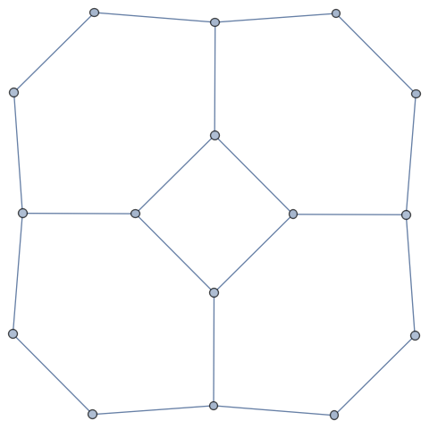
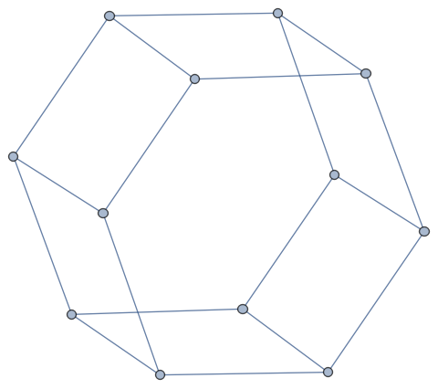
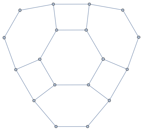
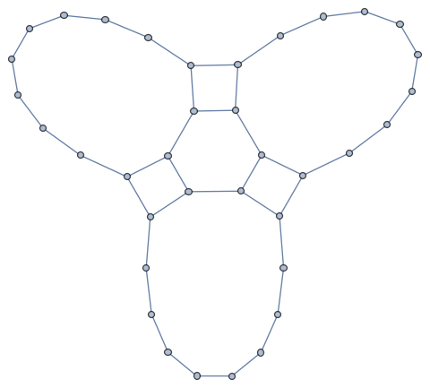
Sectional curvature of x is just defined as the sum of all the and then divided by 3. The reason is that because every vertex degree in the dual graph at is 3, that when adding up all sectional curvatures along a geodesic sheet we count every three times. Here are three examples obtained by taking a host graph . The sectional curvatures are 1/3,2/3 and 1/2. In this case, we see that all sectional curvatures are positive. Here are pictures of the situation near a bone in the case of a 3-dimensional projective plane.
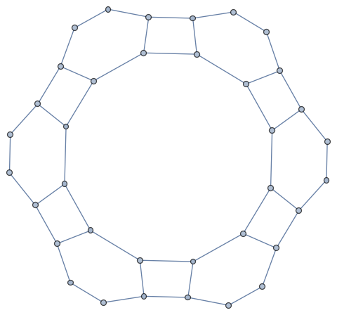
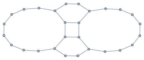
Below are examples for , the two dimensional torus. All sectional curvatures are zero.


 = 1-3/2+1/a_j + 1/b_j + 1/c_j")

 =1-d(x)/2 + \sum_{i=1}^{d(x)} 1/d(F_i)")
=3")
")
/6")
/6>0")


")