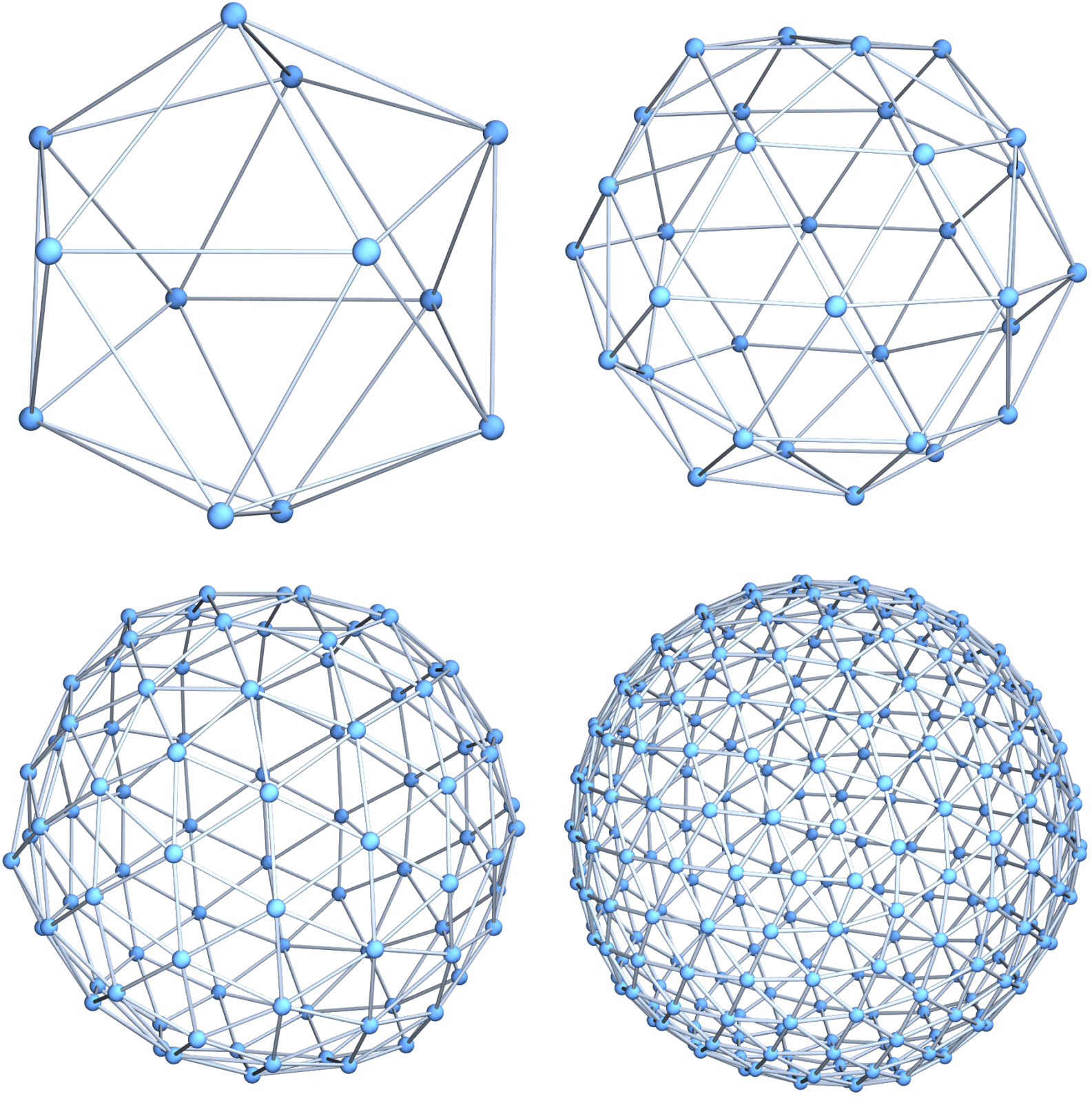
There is a soft Barycentric refinement of graphs or simplicial complexes which can be seen as the usual Barycentric refinement in which the second highest dimensional simplices are collapsed. It is a triangulation of the dual complex. The soft Barycentric refinement of a d-dimensional cross polytop for example is a triangulation of a d-dimensional cube (d-dimensional tesseract). The soft Barycentric refinement of the 16 cell for example is a triangulation of the tesseract. This is handy since we want to deal with duality and also want triangulations. The cube or dodecahedron are not 2-manifolds in the sense that the unit spheres are circular graphs (it needs concept of CW complexes which for various reasons is an enormous jump, first of all pedagogically as CW complexes are introduced usually only in algebraic topology, while graphs already in high school, and then also philosophically as CW complexes come with a build up story, which is from the computer science point of view more involved. We like data structures which are static and simplicial complexes (or more generally delta sets) are static and given by a set of sets and a matrix. . The mathematics of triangulated structures (simplicial complexes in particular) are not only much simpler, but also avoid embarrassing pitfalls as described by Lakatos, especially in higher dimensions, where we have less intuition. In two dimensions, the soft Barycentric refinement is especially attractive because the vertex degree does not explode. A consequence is that the law of the Barycentric limit is still a continuous distribution unlike the law of the Barycentric refinement. So what is the soft Barycentric refinement? Instead of taking all simplices, just restrict to all simplices except the second highest ones, then additionally to the usual connections (defined by inclusion) take also connection of facets which intersect in a second highest dimensional simplex. This is where duality comes in. Classicially, the dual structure is a priori just the graph in which the highest dimensional simplices are the vertices and where two are connected if they intersect in a simplex one dimension lower. Obiously, this naive duality does not preserve manifolds. The classical dual of the icosahedron is the dodecahedron, a triangle free graph. The soft Barycentric refinement however of the icosahedron is a triangulation of the dodecahedron. The picture to the right shows the first 3 soft refinements of the icosahedron. The second refinement is also known as the loop refinement, described by Charles Teorell Loop in 1978. One of the problems in HW 6 (PDF) of math 136 of this Fall 2024 deals with soft Barycentric refinement.
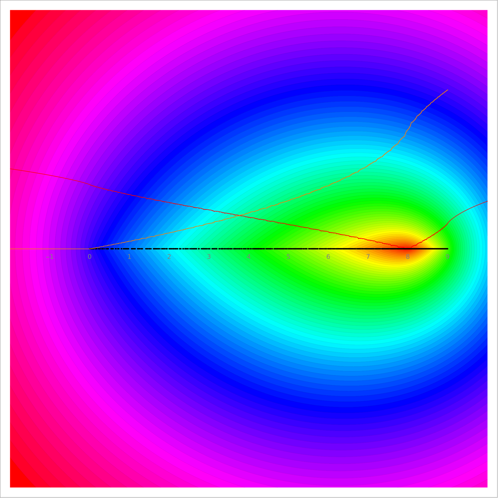
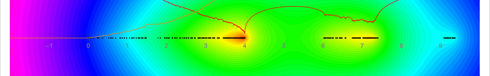
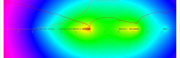
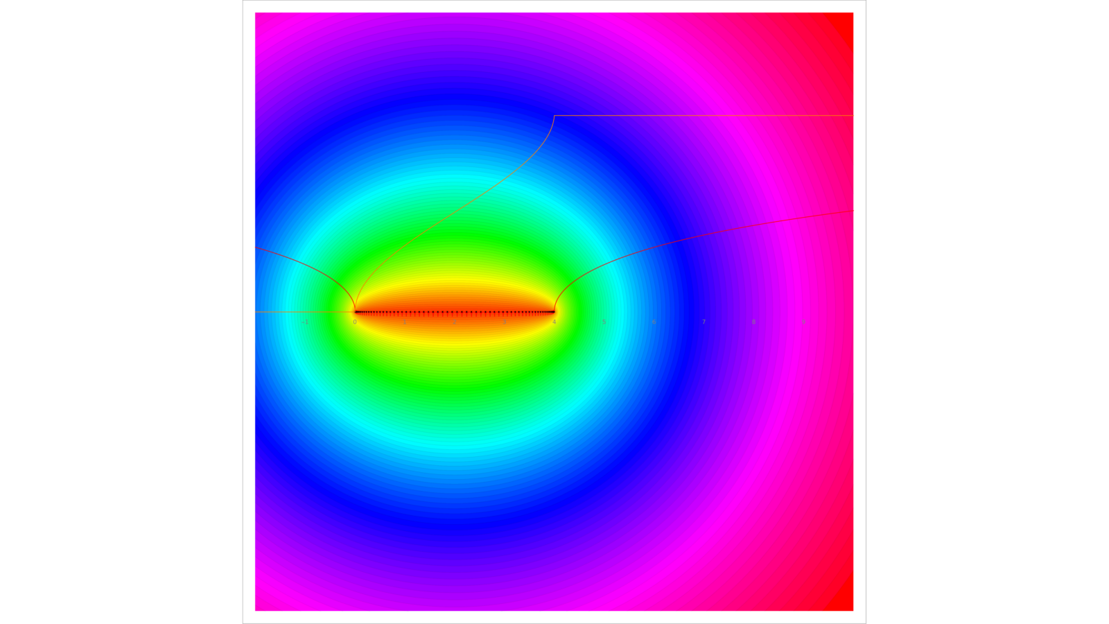
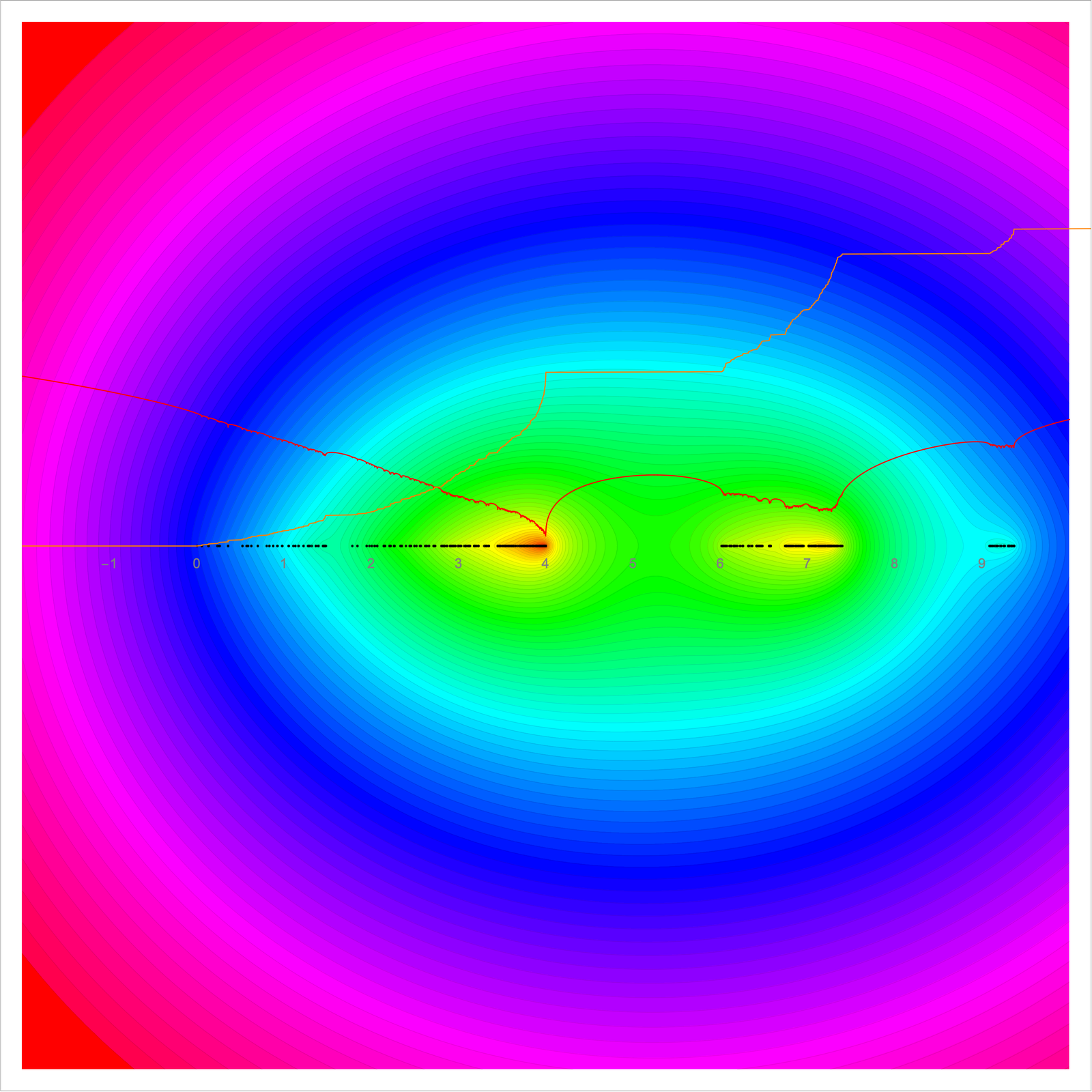
Just to remind about the Barycentric central limit theorem: in that case, there was for every dimension d a limiting universal “law” (density of states) of the Kirchhoff Laplacian (there are similar results for any finite range Laplacian like the Hodge Laplacian or connection Laplacian). Below we see the pictures of the Barycentric universal law in one and two dimensions. The one-dimensional case is completely understood, as it is the equilibrium measure on [0,4] and the arc sin distribution there. The two dimensional case is not understood. It shows Cantor type spectrum. I battled with the potential theoretic properties for a while and showed that the potential values at 0 give the growth rate of the number of spanning trees and the potential value at -1 the growth rate of the number of spanning forests and the tree forest ratio is defined. In order to establish this, I needed to estimate the tail distribution of the density of states (a measure of non-compact support) which needed to estimate all eigenvalues of the Kirchhoff Laplacian. This led to this paper. What happens in the soft Barycentric refinement case is that the 2 dimensional case becomes “integrable” in the sense that one can give the density of states explicitly (it is piecewise linear but I did not prove that yet, it is probably just a simple Fourier picture computation (we need to use characteristic functions as custom in stats to understand distributions.). Below ar the pictures of the distributions of the Barycentral central limit theorem in dimension 1 and 2. in each case, I also drew the potential function (Lyapunov exponent). I’m fond of this stuff because it occupied me for more than a decade in my unsuccessful quest to solve the mystery of positive entropy of dynamical systems like the Standard map. The integrated Lyapunov exponent (by Pesin equal to the Kolmogorov-Sinai entropy) is just the potential value of the zero energy of a random Jacobi matrix (random in the sense of probability theory, where every function on on a probability space is called a random variable). The Hessian of the variational problem of the Standard map is a “non-commutative random variable”, there is nothing a priori random associated to it. That “chaos story” shows that finding potential values of complicated measures in the complex plane can be very hard. The Tree or Forest numbers are no different. In some cases (integrable cases), we can compute it, in most cases not. The soft Barycentric refinement story shifts the dimension of integrability a bit as the two dimensional case is now still integrable. Of course, in three dimensions, where the soft Barycentric refinement will lead to an explosion of vertex degrees the universal limiting measure looks Cantor like again. By the way, that was just the point of this talk: to point out that the Soft Barycentric limit story is mathematically very similar to the Barycentric limit story. The Lidskii-Last tool to establish convergence still also works in the soft Barycentric case.
One of the nice things about the Soft Barycentric refinement, I had cut out in the video. One can get to the limit also by starting with tori. I like the discrete Clifford torus, a 2-dimensional manifold in which every vertex has a circular 
Unlike stated in my presentation, the pictures show potential and not the density. The potential appears to be piecewise linear on the spectrum with a zero at 8. The density of states is maximal of at 8. This is still all only experimental.